Setup
Overview
Teaching: min
Exercises: minQuestions
Objectives
Install necessary software for this workshop
Download data and other setup files for this workshop
Get context of data used in this workshop
Confirm I have the previous knowledge necessary to participate in this workshop
Software setup
FIXME add/edit install instructions (automated, see comment)
Text Editor
When you're writing code, it's nice to have a text editor that is optimized for writing code, with features like automatic color-coding of key words. The default text editor on macOS and Linux is usually set to Vim, which is not famous for being intuitive. If you accidentally find yourself stuck in it, hit the Esc key, followed by :+Q+! (colon, lower-case 'q', exclamation mark), then hitting Return to return to the shell.
nano is a basic editor and the default that instructors use in the workshop. It is installed along with Git.
nano is a basic editor and the default that instructors use in the workshop. See the Git installation video tutorial for an example on how to open nano. It should be pre-installed.
Video Tutorial
nano is a basic editor and the default that instructors use in the workshop. It should be pre-installed.
R
R is a programming language that is especially powerful for data exploration, visualization, and statistical analysis. To interact with R, we use RStudio.
Install R by downloading and running this .exe file from CRAN. Also, please install the RStudio IDE. Note that if you have separate user and admin accounts, you should run the installers as administrator (right-click on .exe file and select "Run as administrator" instead of double-clicking). Otherwise problems may occur later, for example when installing R packages.
Video Tutorial
Install R by downloading and running this .pkg file from CRAN. Also, please install the RStudio IDE.
Video Tutorial
Instructions for R installation on various Linux platforms (debian,
fedora, redhat, and ubuntu) can be found at
<https://cran.r-project.org/bin/linux/>. These will instruct you to
use your package manager (e.g. for Fedora run
sudo dnf install R and for Debian/Ubuntu, add a ppa
repository and then run sudo apt-get install r-base).
Also, please install the
RStudio IDE.
Install the videoconferencing client
If you haven't used Zoom before, go to the official website to download and install the Zoom client for your computer.
Set up your workspace
Like other Carpentries workshops, you will be learning by "coding along" with the Instructors. To do this, you will need to have both the window for the tool you will be learning about (a terminal, RStudio, your web browser, etc..) and the window for the Zoom video conference client open. In order to see both at once, we recommend using one of the following set up options:
- Two monitors: If you have two monitors, plan to have the tool you are learning up on one monitor and the video conferencing software on the other.
- Two devices: If you don't have two monitors, do you have another device (tablet, smartphone) with a medium to large sized screen? If so, try using the smaller device as your video conference connection and your larger device (laptop or desktop) to follow along with the tool you will be learning about.
- Divide your screen: If you only have one device and one screen, practice having two windows (the video conference program and one of the tools you will be using at the workshop) open together. How can you best fit both on your screen? Will it work better for you to toggle between them using a keyboard shortcut? Try it out in advance to decide what will work best for you.
Setup files:
Please download the following files to particpate in the workshop:
FIXME data:
script: R-INTERMEDIATE script
FIXME add links to setup files in files folder OR if there are many files, zip setup files, add to files folder
and add link to zip file here
About the Data Used in this Workshop:
(if the workshop uses data)
FIXME add intro/description of data. Including file format and any disciplinary background needed to understand why the data is gathered and how it is used.
Key Points
Install X software
Install Y software
Download data/setup files x,y,z
Workshop data is from x, in y format and includes x,y,z types of data
Introduction
Overview
Teaching: 0 min
Exercises: 0 minQuestions
Key question (FIXME)
Objectives
First learning objective. (FIXME)
FIXME
Key Points
First key point. Brief Answer to questions. (FIXME)
Functions
Overview
Teaching: min
Exercises: minQuestions
Objectives
Understand the use of functions in R
Understand how to use built in functions in R
Understand how to create your own functions in R
FUNCTIONS
Function arelines of codes which are executed in a sequential order in order to perform a certain task. In other words, it is a set of statements which are executed together to accomplish a certain task. R like any programming language, has many built in functions (also called pre-defined functions) but also allows users to create their own functions which are known as user defined functions.
BUILT IN FUNCTIONS
These are functions which are built inside R which are readily available for all users with access to R.
E.g.:
seq()-Print a sequence of numbers
mean()-Find the mean value of a set of numbers
sum()-Find the sum of a set of numbers
seq(25,35)
results in:
[1] 25 26 27 28 29 30 31 32 33 34 35
You can refer Link1[FIXME link] & Link2 [FIXME link] for some of the most frequently used bult in R functions.
USER DEFINED FUNCTION
These are functions which are manually defined by user and are not available in R by default. Users can create a function based on their own requirements. These functions are useful when a block of code is required to be performed repetitively.
Syntax:
function_name <- function(argument1,argument2, .............)
  {
  Body of the function (or) statements
  return()
  }
Calling the function:
function_name()
Key Points
First key point. Brief Answer to questions. (FIXME)
Data Visualization in R
Overview
Teaching: 0 min
Exercises: minQuestions
Objectives
Understand how to use Base R for plotting.
Learn how to make boxplots and barplots.
In R data can be visualized using the basic plot function. The syntax for the plot command is as below:
plot(data)
Before proceeding ahead kindly load the mtcars data using the below commands:
library(datasets)
data("mtcars")
mtcars$cyl <-as.factor(mtcars$cyl)
mtcars$vs <-as.factor(mtcars$vs)mtcars$am <-as.factor(mtcars$am)
mtcars$gear <-as.factor(mtcars$gear)
mtcars$carb <-as.factor(mtcars$carb)
levels(mtcars$am) <-c(levels(mtcars$am), "Automatic", "Manual")
mtcars$am[mtcars$am == 0]<-"Automatic"
mtcars$am[mtcars$am == 1] <-"Manual"
mtcars$am <-factor(mtcars$am)
str(mtcars)
The plot function creates the plots as below based on data type:
| Plot | Data Type |
|---|---|
| Bar plot | Factor |
| Scattor plot | Numeric |
[FIXME add image plot)mtcars$am) & plot(mtcars$disp)
Barplot
To create a barplot in R we can use the barplot()command, but the data passed to the function must of a table type which contains the count of each factor. [FIXME add image tab <-table]
Syntax:
You can create a better plot using the below arguments:
barplot(data,         # Data in the form of a table
        main = ,      # The heading of the plot
        xlab= ,       # The x-axis label
        ylab = ,      # The y-axis label
        col = )       # Color of the bar
[FIXME add barplot images]
To compare the counts of two different factors the above syntax says the same, only the data passed into the barplot() function is now a table of two factors.
The legend()function can be used to include a legend in the plots but MUST be run immediately after the plot command.
Syntax:
Legend (location_of_legend, legend = legend_keys, fill = colors_of_the_keys)
[FIXME add image # Two Factors]
HISTOGRAM
A histogram is similar to a barplotbut is used for numeric data types. Instead of counting the occurrence of each individual value, a histogram divides the data into bins (buckets/ranges) depending on the entire data range and displays the count.
Syntax:
hist(data, main = “Plot Heading”, xlab = “X-Axis Label”, ylab = “Y-Axis Label”, col = “Bar color”)
[FIXME add image hist() on horse-power distribution]
From the plot we can determine:
- Horsepower range in dataset-50 to 350
- Cars with horsepower between 50 to 100-9
- Cars with horsepower between 100 to 150-10
Thus, a histogram gives an idea about the distribution of the numeric variable in our dataset.
PIE CHART
Pie-Chart is used for the same conditions as a bar chart but is mostly when it is required to show dominance of one or two particular value(s) in comparison with others.
Syntax:
pie(data,       # Data in form of a table
    col = ,     # Colors of the pie slices
    main = )    # Plot heading
[FIXME add image pie chart]
BOX PLOT
A Box Plot is used to understand the distribution of numerical type data in the data set. It helps to understand how data is grouped, if data is skewed and identify the outliers in the data.
[FIXME add image boxplot towardsdatascience]
A boxplot represents data in the below categories: Minimum -Mean –(2 X Standard Deviation) Q1 -25thPercentile Median -50thPercentile Q3 -75thPercentile Maximum -Mean + (2 X Standard Deviation) Outlier -The 0.7% of the data which are more than 2 Standard deviations away from mean.
Kindly find a video explaining in detail percentiles here [FIXME add link] https://www.youtube.com/watch?v=IFKQLDmRK0Y.
A Box Plot can be related to a normal distribution as shown below:
[FIXME add image boxplot vs norm distribution]
Syntax:boxplot(data,boxplot(main =,boxplot(ylab = ,boxplot(col =)Numerical data (or) column fora data framePlot TitleY-Axis LabelColor of the plot
[FIXME add image boxplot horse power]
Boxplot can also be used to analyze the distribution of data across various factors in a column. [FIXME add box plot horsepower/car type]
SCATTER PLOT
Scatter plot can be used to identify if any relationship exists between two numeric variables.
Syntax:
plot(Numerical_column1,     # Column of numerical data type along X-axis
     Numerical_column2,     # Column of numerical data type along Y-axis
     main = ,               # Plot Title
     xlab = ,               # X-Axis Label
     ylab = ,               # Y-Axis Label
     col = )                # Plot Color
[FIXME add image scatter plot]
It can be seen from the plot that as the Horse-Power of the car increased the car Mileage decreases.
Key Points
First key point. Brief Answer to questions. (FIXME)
Hypothesis Testing
Overview
Teaching: min
Exercises: minQuestions
Objectives
What is Hypothesis Testing?
Hypothesis testing is performed to identify if there is a relationship between the attributes (columns) of our data set.
Hypothesis testing is only used to confirm that there is a relation between the attributes considered but does not define the nature of the relationship.
To perform hypothesis testing, we first initially form 2 different hypotheses:
- Null Hypothesis
- No difference between data considered
- Alternate Hypothesis
- There is a difference between the data considered
For example, if we want to perform a hypothesis testing to check if a car’s transmission type (Manual or Automatic) has an impact on the price of a car then our hypothesis would be:
- Null Hypothesis
- There is no difference in the price range of a car based on its type of transmission
- Alternate Hypothesis
- There is a statistical difference in the price range of a car based on its type of transmission
Kindly find a video explaining hypothesis testing in more detail here.
CONFIDENCE INTERVAL
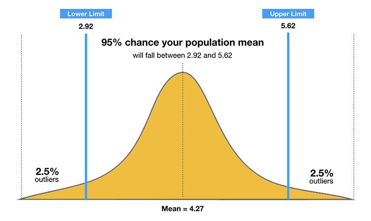
The confidence interval determines the range of values which the true mean lies. For example, if data is collected regarding the height of men then, a 95% confidence interval provides the range of height within which the true mean of all men’s height lie.
P-Value
The p-value of a test provides the probability of gaining results in the extreme cases under the assumption that the null hypothesis is correct. If a p-value is large,then the probability of such a result is very high and if p-value is low then the probability of such a result is very low under the considered null hypothesis.
We chose a significance value to determine when to reject the null hypothesis. Conventionally, 0.05 is chosen as the significance level such that if p-value is less the 0.05 then wereject the null hypothesis and accept the alternate hypothesis.
More on Confidence Intervals
You can refer to the below links to learn more in detail:
- Confidence Interval –MathisFun, YouTube [FIXME add in links]
- P-value –StatsDirect, YouTube, YouTube2, Towards_Data_Science
[FIXME add image “true value under null hypothesis”]
T-TEST
The t-test is used to run a hypothesis testing on one (or) two levels of same factor.
Syntax:
t.test(Factor 1,            # Values of the first factor
       Factor 2,            # Values of the second factor
       alternative = )      # Check if factor 1 mean is smaller or greater than factor 2 (optional)
To determine of the transmission type of a car has an impact on its mileage:
# Storing the mileage of Automatic & Manual transmission cars in individual vectors
Auto_mileage <- mtcars[mtcars$am == "Automatic","mpg"]
Manual_mileage <- mtcars[mtcars$am == "Manual","mpg"]

# T-test to check if transmission type has an effect on the car's mileage
t.test(Auto_mileage, Manual_mileage)
	Welch Two Sample t-test

data:  Auto_mileage and Manual_mileage
t = -3.7671, df = 18.332, p-value = 0.001374
alternative hypothesis: true difference in means is not equal to 0
95 percent confidence interval:
 -11.280194  -3.209684
sample estimates:
mean of x mean of y
 17.14737  24.39231
See the p-value on line 3 of your output:
t = -3.7671, df = 18.332, p-value = 0.001374
Since the p-value is less than 0.05 we can accept the alternate hypothesis that there is a difference in the mileage of a car based on its transmission type.
We can then use the alternative parameter to determine if the first factor under consideration has a higher mean compared to the second factor.
# Is the mileage of the automatic transmission less than the mileage of manual transmission?
t.test(Auto_mileage, Manual_mileage, alternative = "less")
	Welch Two Sample t-test

data:  Auto_mileage and Manual_mileage
t = -3.7671, df = 18.332, p-value = 0.0006868
alternative hypothesis: true difference in means is less than 0
95 percent confidence interval:
      -Inf -3.913256
sample estimates:
mean of x mean of y
 17.14737  24.39231
# Or, is the mileage of the automatic transmission greater than the mileage of manual transmission?
t.test(Auto_mileage, Manual_mileage, alternative = "greater")
	Welch Two Sample t-test

data:  Auto_mileage and Manual_mileage
t = -3.7671, df = 18.332, p-value = 0.9993
alternative hypothesis: true difference in means is greater than 0
95 percent confidence interval:
 -10.57662       Inf
sample estimates:
mean of x mean of y
 17.14737  24.39231
From the test and the resulting p-value(s) we can verify that a car with an Automatic transmission has a lower mileage in comparison to manual transmission carin the dataset.
p-value of less:
t = -3.7671, df = 18.332, p-value = 0.9993
vs.
p-value of greater:
t = -3.7671, df = 18.332, p-value = 0.9993
Ok, now let’s check the impact of transmission type on horsepower:
# T-test to check if transmission type has an effect on the car's horsepower
Auto_hp <- mtcars[mtcars$am == "Automatic","hp"]
Manual_hp <- mtcars[mtcars$am == "Manual","hp"]
t.test(Auto_hp, Manual_hp)
	Welch Two Sample t-test

data:  Auto_mileage and Manual_mileage
t = -3.7671, df = 18.332, p-value = 0.9993
alternative hypothesis: true difference in means is greater than 0
95 percent confidence interval:
 -10.57662       Inf
sample estimates:
mean of x mean of y
 17.14737  24.39231
Since the p-value is greater than 0.05 we can accept the null hypothesis that there is no difference in the horsepower of a car based on its transmission type.
ANOVA
The ANOVA test is performed to run hypothesis testing on a factor with more than two levels. In our mtcarsdataset the “cylinder” attribute has three levels while “carburetors” attribute hassix levels.
Syntax:
# initial anova test
aov(Numerical_column_name~ Categorical_column_name,
    data =dataframe_name)

# tukey test to check for diffence in individual levels
TukeyHSD(ANOVA_output)
The initial anova test only provides a result stating if there is an overall difference.To checkfor difference between each individual level in the factor we use the TukeyHSD() function.
# Test performed to see if mileage varies based on number of cylinders
mileage.aov <- aov(mpg~cyl, data=mtcars)

# The below summary provides a single result indicating if mileage
# varies or not
summary(mileage.aov)

# The TukeyHSD function provides results to indicate if mileage varies
# between each type of cylinder
TukeyHSD(mileage.aov)
> # Test performed to see if mileage varies based on number of cylinders
> mileage.aov <- aov(mpg~cyl, data=mtcars)
>
> # The below summary provides a single result indicating if mileage
> # varies or not
> summary(mileage.aov)
            Df Sum Sq Mean Sq F value   Pr(>F)
cyl          2  824.8   412.4    39.7 4.98e-09 ***
Residuals   29  301.3    10.4
---
Signif. codes:  0 ‘***’ 0.001 ‘**’ 0.01 ‘*’ 0.05 ‘.’ 0.1 ‘ ’ 1
>
> # The TukeyHSD function provides results to indicate if mileage varies
> # between each type of cylinder
> TukeyHSD(mileage.aov)
  Tukey multiple comparisons of means
    95% family-wise confidence level

Fit: aov(formula = mpg ~ cyl, data = mtcars)

$cyl
          diff        lwr        upr     p adj
6-4  -6.920779 -10.769350 -3.0722086 0.0003424
8-4 -11.563636 -14.770779 -8.3564942 0.0000000
8-6  -4.642857  -8.327583 -0.9581313 0.0112287
Based on p-value there seems the be a significant difference in mileage between Cars with:
- 6 & 4 cylinders
- 8 & 4 cylinders
- 6 & 8 cylinders
Now let’s use the ANOVA functions on number of carburetors and horsepower.
# Test performed to see if horse power varies based on number of carburetors
horsepower.
aov <- aov(hp~carb, data=mtcars)
summary(horsepower.aov)
TukeyHSD(horsepower.aov)
Based on p-value there seems the be a significant difference in horse power between Cars with:
- 4 & 1 carburetors
- 8 & 1 carburetors
- 4 & 2 carburetors
- 8 & 2 carburetors
# Test performed to see if horse power varies based on number of carburetors
> horsepower.aov <- aov(hp~carb, data=mtcars)
> summary(horsepower.aov)
            Df Sum Sq Mean Sq F value   Pr(>F)
carb         5  90319   18064   8.476 7.31e-05 ***
Residuals   26  55408    2131
---
Signif. codes:  0 ‘***’ 0.001 ‘**’ 0.01 ‘*’ 0.05 ‘.’ 0.1 ‘ ’ 1
> TukeyHSD(horsepower.aov)
  Tukey multiple comparisons of means
    95% family-wise confidence level

Fit: aov(formula = hp ~ carb, data = mtcars)

$carb
     diff          lwr      upr     p adj
2-1  31.2  -38.6970658 101.0971 0.7429980
3-1  94.0   -3.8754692 191.8755 0.0650833
4-1 101.0   31.1029342 170.8971 0.0018434
6-1  89.0  -62.6280249 240.6280 0.4809394
8-1 249.0   97.3719751 400.6280 0.0003888
3-2  62.8  -30.5672469 156.1672 0.3347215
4-2  69.8    6.3694463 133.2306 0.0248797
6-2  57.8  -90.9578343 206.5578 0.8357649
8-2 217.8   69.0421657 366.5578 0.0015865
4-3   7.0  -86.3672469 100.3672 0.9998994
6-3  -5.0 -168.7769853 158.7770 0.9999988
8-3 155.0   -8.7769853 318.7770 0.0713126
6-4 -12.0 -160.7578343 136.7578 0.9998557
8-4 148.0   -0.7578343 296.7578 0.0517459
8-6 160.0  -40.5850229 360.5850 0.1760952
Correlation Test
The correlation test is used to run a hypothesis testing on two different numerical attributes.
Syntax:
cor.test(Numerical_Attribute_1,
        Numerical_Attribute_2)
# Checking if a relationship exists between mileage and horsepower
cor.test(mtcars$mpg, mtcars$hp)

# Using options command to expand exponent into decimal form
options(scipen = 99)
cor.test(mtcars$mpg, mtcars$hp)

# Checking if a relationship exists between quarter mile time
# and car weight
cor.test(mtcars$qsec, mtcars$wt)
> # Checking if a relationship exists between mileage and horsepower
> cor.test(mtcars$mpg, mtcars$hp)

	Pearson's product-moment correlation

data:  mtcars$mpg and mtcars$hp
t = -6.7424, df = 30, p-value = 1.788e-07
alternative hypothesis: true correlation is not equal to 0
95 percent confidence interval:
 -0.8852686 -0.5860994
sample estimates:
       cor
-0.7761684

>
> # Using options command to expand exponent into decimal form
> options(scipen = 99)
> cor.test(mtcars$mpg, mtcars$hp)

	Pearson's product-moment correlation

data:  mtcars$mpg and mtcars$hp
t = -6.7424, df = 30, p-value = 0.0000001788
alternative hypothesis: true correlation is not equal to 0
95 percent confidence interval:
 -0.8852686 -0.5860994
sample estimates:
       cor
-0.7761684

>
> # Checking if a relationship exists between quarter mile time
> # and car weight
> cor.test(mtcars$qsec, mtcars$wt)

	Pearson's product-moment correlation

data:  mtcars$qsec and mtcars$wt
t = -0.97191, df = 30, p-value = 0.3389
alternative hypothesis: true correlation is not equal to 0
95 percent confidence interval:
 -0.4933536  0.1852649
sample estimates:
       cor
-0.1747159
From the results we can determine that there exists a relationship between mileage and horsepower but no relationship between the car’s weight and quarter mile time (qsec).
Key Points
First key point. Brief Answer to questions. (FIXME)