Hypothesis Testing
Overview
Teaching: min
Exercises: minQuestions
Objectives
What is Hypothesis Testing?
Hypothesis testing is performed to identify if there is a relationship between the attributes (columns) of our data set.
Hypothesis testing is only used to confirm that there is a relation between the attributes considered but does not define the nature of the relationship.
To perform hypothesis testing, we first initially form 2 different hypotheses:
- Null Hypothesis
- No difference between data considered
- Alternate Hypothesis
- There is a difference between the data considered
For example, if we want to perform a hypothesis testing to check if a car’s transmission type (Manual or Automatic) has an impact on the price of a car then our hypothesis would be:
- Null Hypothesis
- There is no difference in the price range of a car based on its type of transmission
- Alternate Hypothesis
- There is a statistical difference in the price range of a car based on its type of transmission
Kindly find a video explaining hypothesis testing in more detail here.
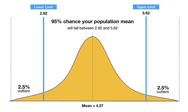
CONFIDENCE INTERVAL
The confidence interval determines the range of values which the true mean lies. For example, if data is collected regarding the height of men then, a 95% confidence interval provides the range of height within which the true mean of all men’s height lie.
P-Value
The p-value of a test provides the probability of gaining results in the extreme cases under the assumption that the null hypothesis is correct. If a p-value is large,then the probability of such a result is very high and if p-value is low then the probability of such a result is very low under the considered null hypothesis.
We chose a significance value to determine when to reject the null hypothesis. Conventionally, 0.05 is chosen as the significance level such that if p-value is less the 0.05 then wereject the null hypothesis and accept the alternate hypothesis.
More on Confidence Intervals
You can refer to the below links to learn more in detail:
- Confidence Interval –MathisFun, YouTube [FIXME add in links]
- P-value –StatsDirect, YouTube, YouTube2, Towards_Data_Science
[FIXME add image “true value under null hypothesis”]
T-TEST
The t-test is used to run a hypothesis testing on one (or) two levels of same factor.
Syntax:
t.test(Factor 1,            # Values of the first factor
       Factor 2,            # Values of the second factor
       alternative = )      # Check if factor 1 mean is smaller or greater than factor 2 (optional)
To determine of the transmission type of a car has an impact on its mileage:
# Storing the mileage of Automatic & Manual transmission cars in individual vectors
Auto_mileage <- mtcars[mtcars$am == "Automatic","mpg"]
Manual_mileage <- mtcars[mtcars$am == "Manual","mpg"]

# T-test to check if transmission type has an effect on the car's mileage
t.test(Auto_mileage, Manual_mileage)
	Welch Two Sample t-test

data:  Auto_mileage and Manual_mileage
t = -3.7671, df = 18.332, p-value = 0.001374
alternative hypothesis: true difference in means is not equal to 0
95 percent confidence interval:
 -11.280194  -3.209684
sample estimates:
mean of x mean of y
 17.14737  24.39231
See the p-value on line 3 of your output:
t = -3.7671, df = 18.332, p-value = 0.001374
Since the p-value is less than 0.05 we can accept the alternate hypothesis that there is a difference in the mileage of a car based on its transmission type.
We can then use the alternative parameter to determine if the first factor under consideration has a higher mean compared to the second factor.
# Is the mileage of the automatic transmission less than the mileage of manual transmission?
t.test(Auto_mileage, Manual_mileage, alternative = "less")
	Welch Two Sample t-test

data:  Auto_mileage and Manual_mileage
t = -3.7671, df = 18.332, p-value = 0.0006868
alternative hypothesis: true difference in means is less than 0
95 percent confidence interval:
      -Inf -3.913256
sample estimates:
mean of x mean of y
 17.14737  24.39231
# Or, is the mileage of the automatic transmission greater than the mileage of manual transmission?
t.test(Auto_mileage, Manual_mileage, alternative = "greater")
	Welch Two Sample t-test

data:  Auto_mileage and Manual_mileage
t = -3.7671, df = 18.332, p-value = 0.9993
alternative hypothesis: true difference in means is greater than 0
95 percent confidence interval:
 -10.57662       Inf
sample estimates:
mean of x mean of y
 17.14737  24.39231
From the test and the resulting p-value(s) we can verify that a car with an Automatic transmission has a lower mileage in comparison to manual transmission carin the dataset.
p-value of less:
t = -3.7671, df = 18.332, p-value = 0.9993
vs.
p-value of greater:
t = -3.7671, df = 18.332, p-value = 0.9993
Ok, now let’s check the impact of transmission type on horsepower:
# T-test to check if transmission type has an effect on the car's horsepower
Auto_hp <- mtcars[mtcars$am == "Automatic","hp"]
Manual_hp <- mtcars[mtcars$am == "Manual","hp"]
t.test(Auto_hp, Manual_hp)
	Welch Two Sample t-test

data:  Auto_mileage and Manual_mileage
t = -3.7671, df = 18.332, p-value = 0.9993
alternative hypothesis: true difference in means is greater than 0
95 percent confidence interval:
 -10.57662       Inf
sample estimates:
mean of x mean of y
 17.14737  24.39231
Since the p-value is greater than 0.05 we can accept the null hypothesis that there is no difference in the horsepower of a car based on its transmission type.
ANOVA
The ANOVA test is performed to run hypothesis testing on a factor with more than two levels. In our mtcarsdataset the “cylinder” attribute has three levels while “carburetors” attribute hassix levels.
Syntax:
# initial anova test
aov(Numerical_column_name~ Categorical_column_name,
    data =dataframe_name)

# tukey test to check for diffence in individual levels
TukeyHSD(ANOVA_output)
The initial anova test only provides a result stating if there is an overall difference.To checkfor difference between each individual level in the factor we use the TukeyHSD() function.
# Test performed to see if mileage varies based on number of cylinders
mileage.aov <- aov(mpg~cyl, data=mtcars)

# The below summary provides a single result indicating if mileage
# varies or not
summary(mileage.aov)

# The TukeyHSD function provides results to indicate if mileage varies
# between each type of cylinder
TukeyHSD(mileage.aov)
> # Test performed to see if mileage varies based on number of cylinders
> mileage.aov <- aov(mpg~cyl, data=mtcars)
>
> # The below summary provides a single result indicating if mileage
> # varies or not
> summary(mileage.aov)
            Df Sum Sq Mean Sq F value   Pr(>F)
cyl          2  824.8   412.4    39.7 4.98e-09 ***
Residuals   29  301.3    10.4
---
Signif. codes:  0 ‘***’ 0.001 ‘**’ 0.01 ‘*’ 0.05 ‘.’ 0.1 ‘ ’ 1
>
> # The TukeyHSD function provides results to indicate if mileage varies
> # between each type of cylinder
> TukeyHSD(mileage.aov)
  Tukey multiple comparisons of means
    95% family-wise confidence level

Fit: aov(formula = mpg ~ cyl, data = mtcars)

$cyl
          diff        lwr        upr     p adj
6-4  -6.920779 -10.769350 -3.0722086 0.0003424
8-4 -11.563636 -14.770779 -8.3564942 0.0000000
8-6  -4.642857  -8.327583 -0.9581313 0.0112287
Based on p-value there seems the be a significant difference in mileage between Cars with:
- 6 & 4 cylinders
- 8 & 4 cylinders
- 6 & 8 cylinders
Now let’s use the ANOVA functions on number of carburetors and horsepower.
# Test performed to see if horse power varies based on number of carburetors
horsepower.
aov <- aov(hp~carb, data=mtcars)
summary(horsepower.aov)
TukeyHSD(horsepower.aov)
Based on p-value there seems the be a significant difference in horse power between Cars with:
- 4 & 1 carburetors
- 8 & 1 carburetors
- 4 & 2 carburetors
- 8 & 2 carburetors
# Test performed to see if horse power varies based on number of carburetors
> horsepower.aov <- aov(hp~carb, data=mtcars)
> summary(horsepower.aov)
            Df Sum Sq Mean Sq F value   Pr(>F)
carb         5  90319   18064   8.476 7.31e-05 ***
Residuals   26  55408    2131
---
Signif. codes:  0 ‘***’ 0.001 ‘**’ 0.01 ‘*’ 0.05 ‘.’ 0.1 ‘ ’ 1
> TukeyHSD(horsepower.aov)
  Tukey multiple comparisons of means
    95% family-wise confidence level

Fit: aov(formula = hp ~ carb, data = mtcars)

$carb
     diff          lwr      upr     p adj
2-1  31.2  -38.6970658 101.0971 0.7429980
3-1  94.0   -3.8754692 191.8755 0.0650833
4-1 101.0   31.1029342 170.8971 0.0018434
6-1  89.0  -62.6280249 240.6280 0.4809394
8-1 249.0   97.3719751 400.6280 0.0003888
3-2  62.8  -30.5672469 156.1672 0.3347215
4-2  69.8    6.3694463 133.2306 0.0248797
6-2  57.8  -90.9578343 206.5578 0.8357649
8-2 217.8   69.0421657 366.5578 0.0015865
4-3   7.0  -86.3672469 100.3672 0.9998994
6-3  -5.0 -168.7769853 158.7770 0.9999988
8-3 155.0   -8.7769853 318.7770 0.0713126
6-4 -12.0 -160.7578343 136.7578 0.9998557
8-4 148.0   -0.7578343 296.7578 0.0517459
8-6 160.0  -40.5850229 360.5850 0.1760952
Correlation Test
The correlation test is used to run a hypothesis testing on two different numerical attributes.
Syntax:
cor.test(Numerical_Attribute_1,
        Numerical_Attribute_2)
# Checking if a relationship exists between mileage and horsepower
cor.test(mtcars$mpg, mtcars$hp)

# Using options command to expand exponent into decimal form
options(scipen = 99)
cor.test(mtcars$mpg, mtcars$hp)

# Checking if a relationship exists between quarter mile time
# and car weight
cor.test(mtcars$qsec, mtcars$wt)
> # Checking if a relationship exists between mileage and horsepower
> cor.test(mtcars$mpg, mtcars$hp)

	Pearson's product-moment correlation

data:  mtcars$mpg and mtcars$hp
t = -6.7424, df = 30, p-value = 1.788e-07
alternative hypothesis: true correlation is not equal to 0
95 percent confidence interval:
 -0.8852686 -0.5860994
sample estimates:
       cor
-0.7761684

>
> # Using options command to expand exponent into decimal form
> options(scipen = 99)
> cor.test(mtcars$mpg, mtcars$hp)

	Pearson's product-moment correlation

data:  mtcars$mpg and mtcars$hp
t = -6.7424, df = 30, p-value = 0.0000001788
alternative hypothesis: true correlation is not equal to 0
95 percent confidence interval:
 -0.8852686 -0.5860994
sample estimates:
       cor
-0.7761684

>
> # Checking if a relationship exists between quarter mile time
> # and car weight
> cor.test(mtcars$qsec, mtcars$wt)

	Pearson's product-moment correlation

data:  mtcars$qsec and mtcars$wt
t = -0.97191, df = 30, p-value = 0.3389
alternative hypothesis: true correlation is not equal to 0
95 percent confidence interval:
 -0.4933536  0.1852649
sample estimates:
       cor
-0.1747159
From the results we can determine that there exists a relationship between mileage and horsepower but no relationship between the car’s weight and quarter mile time (qsec).
Key Points
First key point. Brief Answer to questions. (FIXME)