Setup

Overview

Time: min

Objectives

Software setup

Please install R and RStudio before this workshop or login to the UIC virtual lab to use the software required for the workshop. See instructions below for both options.

Install the videoconferencing client

If you haven't used Zoom before, go to the official website to download and install the Zoom client for your computer.

Set up your workspace

You will have the opportunity to code along with the Instructors. To do this, you will need to have both the window for the tool you will be learning about (a terminal, RStudio, your web browser, etc..) and the window for the Zoom video conference client open. In order to see both at once, we recommend using one of the following set up options:

• Two monitors: If you have two monitors, plan to have the tool you are learning up on one monitor and the video conferencing software on the other.
• Two devices: If you don't have two monitors, do you have another device (tablet, smartphone) with a medium to large sized screen? If so, try using the smaller device as your video conference connection and your larger device (laptop or desktop) to follow along with the tool you will be learning about.
• Divide your screen: If you only have one device and one screen, practice having two windows (the video conference program and one of the tools you will be using at the workshop) open together. How can you best fit both on your screen? Will it work better for you to toggle between them using a keyboard shortcut? Try it out in advance to decide what will work best for you.

Setup files:

Please download the following files to particpate in the workshop:

R Project zip files

About the Data Used in this Workshop:

This workshop uses an adapted version of the data paper: Nitsch, F. J., Sellitto, M., & Kalenscher, T. (2021). The effects of acute and chronic stress on choice consistency. Psychoneuroendocrinology, 131, 105289. https://doi.org/10.1016/j.psyneuen.2021.105289.

The data paper along with its underlying data publicly available at: https://osf.io/6mvq7 were adapted and used for educational purposes with authors’ permission.

Key Points

Introduction to R and R studio

Overview

Time: min

Objectives

• Understand the basics of R and R studio

• learn about the Rstudio Interface

R

R is a specialized language most commonly used for statistical computing, data analysis, and implementing graphics. It is open-source and free. R Language is widely used by statisticians and data miners for developing statistical software and data analysis. It helps to perform data wrangling, analyzing, and visualizing data easily.

Why use R

• R is a very easy and powerful tool for any statistical operations which can also easily be learned by any person even from a non-technical background.
• R offers a variety of packages each of which helps you perform different functions. As of 2021, there are 18839 available packages in R the list of which can be found here.
• R provides a wide variety of statistical (linear and nonlinear modeling, classical statistical tests (e.g., probability, std deviation, etc.), time series analysis, classification, clustering,) and graphical techniques and is highly extensible.

Based on the 2021 survey conducted by Kaggle, R was the third most used programming language by data professionals

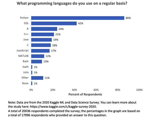
Image Source: Business Broadway, 2021

Understanding R Studio and Console

RStudio is the integrated development environment (IDE) for the basic R software. It is available in two versions:

• RStudio Desktop - Regular desktop application.
• RStudio Server - Runs on a remote server and accessed RStudio using a web browser.

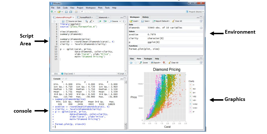
Script Area: - Write codes (or) scripts and run them separately. Also, create a document outline (located on the top right of the script area) in this section that shows all the cod headers in one space.

Console: - Write and run the code together directly here. It also displays the history of any command or an error message in case of a code error.

Environment – List of objects and variables created and present in the current session and also shows the current project file name at the top right of the pane.

Graphics: - Displays the plots, packages, and has an important tab of files. The files option helps us navigate through the different folders of the current project and makes organizing and sorting things a lot better.

The preferences tab in the toolbar helps customize the margins, displays, and font sizes in the r studio.

Help and Cheatsheets in RStudio

help(function_name) – Provides detailed description of function in help window (bottom right) E.g., Run the command help(sort) in the console.

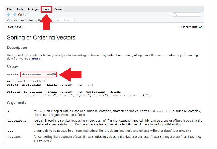
You will now get a complete description of the “sort” function in the help window Points to note:

• If a function’s argument is not given any value (such as x in the above picture) in the help description, this value must be compulsorily specified while running the function
• If a function’s argument is given a value (decreasing = FALSE in above pic) this value is the default value considered by R. It needs to be specified compulsorily when the argument’s value needs to be different.

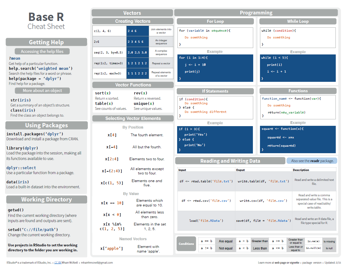
Cheatsheet – In the wild and woolly world of R there are many packages and to summarize this package functions the cheat sheets come in handy. These cheat sheets are invaluable as learning tools. RStudio has created a large number of cheat sheets, including the one-page R Markdown cheat sheet, which is freely available here

Key Points

R syntax and operators

Overview

Time: 0 min

Objectives

• perform basic arithematic functions

• Understand the basic logical operators

R syntax and Logical operators

Codes can be directly run in the R console. Try running the below code to perform basic arithmetic operations of Addition (+), Subtraction (-), Multiplication (*), Division (/) and Modulo (%%) operation directly in the console.

 > 2+2
 [1] 4
 > 2-2
 [1] 0
 >2*2
 [1] 4
 > 2/2
 [1] 1
 > 3%%2
 [1] 1

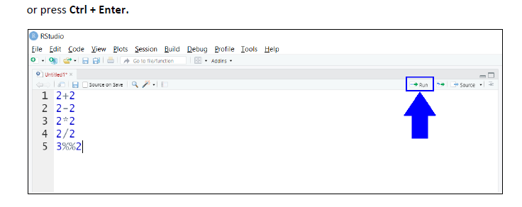
Implementing the same code in the script area. If you do not see a file open in the script area select File → New File → R Script from the menu and then type the code in the new file that appears. Now the code in the script area (or R File) does not execute automatically, instead place the cursor on the line which needs to be executed and select RUN option or press Ctrl + Enter(for windows). To run multiple lines of code, select all the lines first and then select RUN option or press Ctrl + Enter.

Values can be assigned to variables in R using the “<-” symbol. The variable is written on the left and is assigned the value on the right side. For example, to assign a value of 3 to x we can type the below code, x <- 3

Assigning values to variables are quite useful especially if these values would be used again. Similar to the previous examples, operations can be performed on the variables to get output directly (or) the output can be stored in a different variable. Once a variable is created it will be visible under the environment section

> x <- 3
> y <- 5
> x+y
[1] 8
> z <- x+y
> z
[1] 8

One thing to be aware of is that R is case-sensitive. Hence variable “a” is different from “A”

LOGICAL OPERATORS

Provides a list of Boolean results based on operation performed

• < Less than

• <= Less than or equal to

• > Greater than

• >= Greater than or equal to

• == Equal to

• ! = Not equal to

• x&y AND operation

• x|y OR operation

• !x NOT operation

Please note that in R the Boolean values “TRUE” & “FALSE” can also be written as “T” &” F”.

Function in R

A key feature of R is functions. Functions are “self contained” modules of code that accomplish a specific task. Functions usually take in some sort of data structure (value, vector, dataframe etc.), process it, and return a result. The general usage for a function is the name of the function followed by parentheses:function_name(input)

Comments in R

Comments can be used to explain R code, and to make it more readable. It can also be used to prevent execution when testing alternative code. Comments starts with a # When executing the R-code, R will ignore anything that starts with #.

Example:- # This is a comment “Hello World!”

Key Points

Variables and datatypes

Overview

Time: min

Objectives

• understand where to access packages for different functions

• learn about the data types permitted for analysis in R studio

Variables

-It’s a memory location where you store some type of value and where that value can be altered based on your need. Variable is also known as Identifier because the variable name identifies the value that is stored in the memory (RAM). As we Know R is a case-sensitive language hence a variable ABC = 15 and Abc= 32 can have different values.

Naming Variables

• Variable name must start with “letter” and can contain a number, letter, underscore (_) and period (‘.’) ```diff

• variableName1, one.variable ```

• Underscores (_) at the beginning of the variable name is not allowed. ```diff
• _variable_one. ```
• Periods (.) at the beginning of the variable name are allowed but should not be followed by a number eg - ```diff
• .1myvariable ```

• Reserved words or keywords are not allowed to be identified as a variable name.

• Special characters such as “#”, “&’, etc., along with white spaces (tabs, space) are not allowed in a variable name

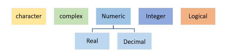
Data Types

Data type in R specifies the size and type of information the variable will store.

R language has five main data types

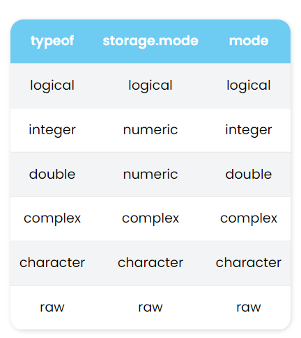
Checking data type in R

There are several functions that can show you the data type of an R object, such as typeof, mode, storage.mode, class and str.the main use of some of them is not to just check the data type of an R object. For instance, the class of an R object can be different from the data type (which is very useful when creating S3 classes) and the str function is designed to show the full structure of an object. If you want to print the R data type, we recommend using the typeof function. To summarize, the following imagwe shows the differences of the possible outputs when applying typeof, storage.mode and mode functions.

There are other functions that allow you to check if some object belongs to some data type, returning TRUE or FALSE. As a rule, these functions start with is. followed by the data type.

Example- is.numeric(4) #true

Data type coercion

You can coerce data types in R with the functions starting with as., summarized

as.numeric == numeric
as.integar == integer 
as.double == double 
as.character == Character
as.logical== Boolean
as.raw ==	 Raw

Character data type

Character data type stores value or strings and contains alphabets, numbers, and symbols

Character data type value is written withing single (‘ ‘)or double inverted quotes (“ “)

Example- “A”, “2.21”, “skill@”.

# input code
# Declaring character value with double quotes ""
charac <- "Abcd"
charac
class(charac)

# Declaring character value with single quotes ''
charac_1 <- 'b'
charac_1
class(charac_1)

#Convert values to character data type.
pi_value <- 3.14
x <- as.character(pi_value)
x
class(x)

# Concatenation of Character
firstname <- "Kasturi "
lastname <- "Acharya"

# Character Value Concatenation
# Paste function is used to concatenate characters
full_name <- paste (firstname, lastname)
full_name

# output
# Declaring character value with double quotes ""
> charac <- "Abcd"
> charac
[1] "Abcd"
> class(charac)
[1] "character"

 # Declaring character value with single quotes ''
> charac_1 <- 'b'
> charac_1
[1] "b"
> class(charac_1)
[1] "character"

> #Convert values to character data type.
> pi_value <- 3.14
> x <- as.character(pi_value)
> x
[1] "3.14"
> class(x)
[1] "character"
> 
> # Concatenation of Character
> first_name <- "Kasturi"
> last_name <- "Acharya"
> 
> # Character Value Concatenation
> # Paste function is used to concatenate characters
> full_name <- paste (first_name,last_name)
> full_name
[1] "Kasturi Acharya"

Complex data type

• R supports a set of all complex numbers and also stores numbers with an imaginary component. Examples: 1+3i, 5i, 5- 9i

# input code
# Assign complex value to x
x <- 10 + 6i + 20
x
class(x)
z <- 6i
z
class(z)

#Using as.complex() function to convert value to complex.
as.complex(5)
as.complex(7i)

# Square root function on complex numbers
#Find the square root of -3+0i
sqrt (-3) 

#Typing in the complete value
sqrt(-1+0i) 

#Coerce to complex value
sqrt (as.complex (-1))


#Performing Addition on Complex Numbers
y1 <- 7+3i
y2 <- 8+9i
sum_y <- y1+y2
sum_y
class(sum_y)

# output
> # Assign complex value to x
> x <- 10 + 6i + 20
> x
[1] 30+6i
> class(x)
[1] "complex"
> z <- 6i
> z
[1] 0+6i
> class(z)
[1] "complex"

> #Using as.complex() function to convert value to complex.
> as.complex(5)
[1] 5+0i
> as.complex(7i)
[1] 0+7i
> 
> # Square root function on complex numbers
> #Find the square root of -3+0i
> sqrt (-3) 
[1] NaN
Warning message:
In sqrt(-3) : NaNs produced
> 
> #Typing in the complete value
> sqrt(-1+0i) 
[1] 0+1i
> 
> #Coerce to complex value
> sqrt (as.complex (-1))
[1] 0+1i
> 
> 
> #Performing Addition on Complex Numbers
> y1 <- 7+3i
> y2 <- 8+9i
> sum_y <- y1+y2
> sum_y
[1] 15+12i
> class(sum_y)
[1] "complex"
> 

Numeric Data Type

• This data type is for numeric values which contain numbers with or without a decimal point,

• This is the default number data type in R

Example: - 1, 20.5, -97.05, -65

# input code
# Assigning a decimal value to variable x
x <- 15.6
x
class(x)
typeof(x)

x1 <- 20
x1
class(x1)
typeof(x1)


# Converting an integer value to numeric type
x2 <- 22L
class(x2)
typeof(x2)
x3 <- as.numeric(x2)
x3
class(x3)
typeof(x3)

# output
> # Assigning a decimal value to variable x
> x <- 15.6
> x
[1] 15.6
> class(x)
[1] "numeric"
> typeof(x)
[1] "double"
> 
> x1 <- 20
> x1
[1] 20
> class(x1)
[1] "numeric"
> typeof(x1)
[1] "double"
> 
> # Converting an integer value to numeric type
> x2 <- 22L
> class(x2)
[1] "integer"
> typeof(x2)
[1] "integer"
> x3 <- as.numeric(x2)
> x3
[1] 22
> class(x3)
[1] "numeric"
> typeof(x3)
[1] "double"

Integer Data Type

• Integer data type stores non-decimal values.

• The as. integer () function can be used to convert a number into integer type data in R.

Example – 5, 102, 600, 1003.

# input code
x <-  18L # putting capital 'L' after a value forces it to be
# stored as Integer.
class(x)


y <-  9
class(y)


x1 <-  23.0L
x1 <-  23L
class(x1)


# Using integer function to declare an Integer type value 
y1 <-  as.integer(44)
class(y1)

#coerce a numeric value into integer
y2 <-  as.integer(45.2)
y2

#Parse a string (coerce a decimal string)
y3 <- as.integer("8.65")
class(y3)

#Convert Logical States to Integer
Logic_True <- as.integer(TRUE)
Logic_True

Logic_False <- as.integer(FALSE)
Logic_False

# To check if the value is integer type:
is.integer(x)
is.integer(y)
is.integer(y1)


#Creating integer vector from 1 to 5
m = 1:5
m
class(m)

# output
> 
> x <-  18L # putting capital 'L' after a value forces it to be
> # stored as Integer.
> class(x)
[1] "integer"
> 
> 
> y <-  9
> class(y)
[1] "numeric"
> 
> 
> x1 <-  23.0L
Warning message:
integer literal 23.0L contains unnecessary decimal point 
> x1 <-  23L
> class(x1)
[1] "integer"
> 
> 
> # Using integer function to declare an Integer type value 
> y1 <-  as.integer(44)
> class(y1)
[1] "integer"
> 
> #coerce a numeric value into integer
> y2 <-  as.integer(45.2)
> y2
[1] 45
> 
> #Parse a string (coerce a decimal string)
> y3 <- as.integer("8.65")
> class(y3)
[1] "integer"
> 
> #Convert Logical States to Integer
> Logic_True <- as.integer(TRUE)
> Logic_True
[1] 1
> 
> Logic_False <- as.integer(FALSE)
> Logic_False
[1] 0
> 
> # To check if the value is integer type:
> is.integer(x)
[1] TRUE
> is.integer(y)
[1] FALSE
> is.integer(y1)
[1] TRUE
> 
> 
> #Creating integer vector from 1 to 5
> m = 1:5
> m
[1] 1 2 3 4 5
> class(m)
[1] "integer"
> 

# input code
# BONUS
#Integers value can be a maximum 2147483647 (2 billion)
.Machine$integer.max 

#Double value can be a maximum 1.797693e+308 (very much > than 2B)
.Machine$double.xmax 

Logical Data Type

• This data type stores logical or Boolean values which are often generated as a result of logical operations.
• Example – True, False

# input code
x <- TRUE
y<- FALSE

x1 <- T
y1 <- F

typeof(x1)
mode(x1)

####################
# Value Comparison #
####################

# Less Than and Greater Than Comparison
32 < 98  # TRUE Statement
37 > 52  # FALSE Statement
87 <= 92 # TRUE Statement
1 >= 9   # FALSE Statement

# Equal TO Comparison
57 == 34  # FALSE Statement
80 == 80  # TRUE Statement
"hi" == "hi" # TRUE Statement

# output
 x <- TRUE
> y<- FALSE
> 
> x1 <- T
> y1 <- F
> typeof(x1)
[1] "logical"
> mode(x1)
[1] "logical"

> # Value Comparison #
>
> # Less Than and Greater Than Comparison
> 32 < 98  # TRUE Statement
[1] TRUE
> 37 > 52  # FALSE Statement
[1] FALSE
> 87 <= 92 # TRUE Statement
[1] TRUE
> 1 >= 9   # FALSE Statement
[1] FALSE
> 
> # Equal TO Comparison
> 57 == 34  # FALSE Statement
[1] FALSE
> 80 == 80  # TRUE Statement
[1] TRUE
> "hi" == "hi" # TRUE Statement
[1] TRUE

Key Points

• importance of using packages in R studio for efficient data analysis

Intoduction to strings and data structures

Overview

Time: min

Objectives

• understand basics of strings and string manipulation

• understanding different data structure

• learn about functions of each data structure

Strings

• Strings are made of a single character or contain a collection of characters.
• Strings can be created by either single quotes (‘ ‘) or double quotes (“ “)

Rule for String in R

• String starts and ends with a single quote. Double quotes (“ “), and through the escape sequence (‘/’), single quote can become a part of the string. Example- ‘buses’, ‘merry”s’, ‘ merry\’s’

• String start and end with a double quote. Single quote (‘ ‘), and through the escape sequence (‘\’), double quote can become a part of the string Example : “buses”, “merry’s”, “ merry\”s”

# input code string concatenation
Count number of characters 
x1 <- "Olivia"
x2 <- "Jhon"
x3 <- "William"

#checking number of characters
nchar(x1)
nchar(x2)
nchar(x3)

# Letters using vector function in R
# Check the sequence of letters
letters
letters[4]
letters[1:5]

# String Concatenation
# Paste function is used with syntax below:

x <- paste("Hello","World","!",sep = " ")
x

y <- paste(x1,x2,x3,"is happy.")
y

z<- paste("Hello","everyone","!", sep =" ")
z
# Vectors

c() # concatenate function

x4 <- c("Olivia","Jhon","William")
y1 <- paste(x4,"is happy.")
y1

z1 <- c("Please bring me","a few ")
z2 <- c("some vegetables","fruits")
z <- paste(z1,z2,collapse = " and ")
z

# output
 # input code string concatenation
> Count number of characters 
Error: unexpected symbol in "Count number"
> x1 <- "Olivia"
> x2 <- "Jhon"
> x3 <- "William"
> 
> #checking number of characters
> nchar(x1)
[1] 6
> nchar(x2)
[1] 4
> nchar(x3)
[1] 7
> 
> # Letters using vector function in R
> # Check the sequence of letters
> letters
 [1] "a" "b" "c" "d" "e" "f" "g" "h" "i" "j" "k" "l" "m" "n" "o" "p" "q" "r" "s" "t" "u" "v" "w" "x"
[25] "y" "z"
> letters[4]
[1] "d"
> letters[1:5]
[1] "a" "b" "c" "d" "e"
> 
> # String Concatenation
> # Paste function is used with syntax below:
> 
> x <- paste("Hello","World","!",sep = " ")
> x
[1] "Hello World !"
> 
> y <- paste(x1,x2,x3,"is happy.")
> y
[1] "Olivia Jhon William is happy."
> 
> z<- paste("Hello","everyone","!", sep =" ")
> z
[1] "Hello everyone !"
> 
> x4 <- c("Olivia","Jhon","William")
> y1 <- paste(x4,"is happy.")
> y1
[1] "Olivia is happy."  "Jhon is happy."    "William is happy."
> 
> z1 <- c("Please bring me","a few ")
> z2 <- c("some vegetables","fruits")
> z <- paste(z1,z2,collapse = " and ")
> z
[1] "Please bring me some vegetables and a few  fruits"

String Manipulation

-it’s the process of corecing, slicing, pasting, or analyzing strings

x <- "William is happy today"
x

# Converting all words to upper case using toupper() function
toupper(x)

# Converting all words to lower case using tolower() function
tolower(x)

x1 <- "Henry is A hardworker. He owns A house and A car."
x1
chartr("A", "a", x1)

z <- "I widd gq tq market tqmqrrqw."
chartr("dq","lo", z)

x2 <- "Henry puts in all his good efforts"
x2
substr(x2, start = 22, stop = 27)

#split function

x4 <- "Henry puts in all his good efforts"
class(x4)
y1 <- strsplit(x4, split = " ")
y1
class(y1)
#either create a variable like y1 or direct use the function in case of Mason 
strsplit("Mason", split ="") 
x4
y2 <- unlist(strsplit(x4, split = " "))
y2
class(y2)

#output 
> x <- "William is happy today"
> x
[1] "William is happy today"
> 
> # Converting all words to upper case using toupper() function
> toupper(x)
[1] "WILLIAM IS HAPPY TODAY"
> 
> # Converting all words to lower case using tolower() function
> tolower(x)
[1] "william is happy today"
> 
> x1 <- "Henry is A hardworker. He owns A house and A car."
> x1
[1] "Henry is A hardworker. He owns A house and A car."
> chartr("A", "a", x1)
[1] "Henry is a hardworker. He owns a house and a car."
> 
> z <- "I widd gq tq market tqmqrrqw."
> chartr("dq","lo", z)
[1] "I will go to market tomorrow."
> 
> x2 <- "Henry puts in all his good efforts"
> x2
[1] "Henry puts in all his good efforts"
> substr(x2, start = 22, stop = 27)
[1] " good "
> 
> #split function
> 
> x4 <- "Henry puts in all his good efforts"
> class(x4)
[1] "character"
> y1 <- strsplit(x4, split = " ")
> y1
[[1]]
[1] "Henry"   "puts"    "in"      "all"     "his"     "good"    "efforts"

> class(y1)
[1] "list"
> #either create a variable like y1 or direct use the function in case of Mason 
> strsplit("Mason", split ="") 
[[1]]
[1] "M" "a" "s" "o" "n"

> x4
[1] "Henry puts in all his good efforts"
> y2 <- unlist(strsplit(x4, split = " "))
> y2
[1] "Henry"   "puts"    "in"      "all"     "his"     "good"    "efforts"
> class(y2)
[1] "character"

Data Structure

A data structure is essentially a way to organize data in a system to facilitate effective usage of the same.Data structures are the objects that are manipulated regularly in R. They are used to store data in an organized fashion to make data manipulation and other data operations more efficient. R has many data structure which are as follows

• Vectors

• Lists

• Matrices

• Factors

• Data Frames

• Arrays

Vector

Vectors are the basic data structure of R. Vectors can hold multiple values together using the concatenate c() function. The type of data inside a vector can be determined by using the type of() function and the length (or) number of elements in a vector can be found with the length() function.

R uses one indexing unlike python, hence the position of the first component in a vector can be accessed by vector name [1]

A vector will always contain data of the same data type. If a vector contains multiple data types the vector will convert all its values to the same data type in the below order of precedence:

• Character

• Double (Float / Decimals)

• Integers (Round whole numbers)

# input code

v1 <- c(1, 2, 3, 4, 5)
v1
is.vector(v1)

v2 <- c("a", "b", "c")
v2
is.vector(v2)

v3 <- c (TRUE, TRUE, FALSE, FALSE, TRUE)
v3
is.vector(v3)

v4<- c (TRUE, TRUE, "a", 5)
v4
typeof(v4)

v5<- c(6,7 ,8.8,23L)
v5
typeof(v5)

# output
> v1 <- c(1, 2, 3, 4, 5)
> v1
[1] 1 2 3 4 5
> is.vector(v1)
[1] TRUE
>
> v2 <- c("a", "b", "c")
> v2
[1] "a" "b" "c"
> is.vector(v2)
[1] TRUE
>
> v3 <- c (TRUE, TRUE, FALSE, FALSE, TRUE)
> v3
[1]  TRUE  TRUE FALSE FALSE  TRUE
> is.vector(v3)
[1] TRUE
>
> v4<- c (TRUE, TRUE, "a", 5)
> v4
[1] "TRUE" "TRUE" "a"    "5"   
> typeof(v4)
[1] "character"

> v5<- c(6,7 ,8.8,23L)
> v5
[1]  6.0  7.0  8.8 23.0
> typeof(v5)
[1] "double"

Analyzing a Vector

class(vector_name) - Type of data present inside the vector

str(vector_name) - Structure of the vector

is.na(vector_name) - Checks if each element of vector is “NA”

is.null(vector_name) - Checks if the entire vector is empty

length(vector_name) - Number of elements present inside the vector

> x <- c(1,2,3,4)
> class(x)
[1] "numeric"
> str(x)
 num [1:4] 1 2 3 4
> length(x)
[1] 4
>
> x<- c(1,2,3,4)
> is.na(x)
[1] FALSE FALSE FALSE FALSE
> is.null(x)
[1] FALSE
>
> x<- c(TRUE, FALSE, TRUE, TRUE)
> class(x)
[1] "logical"
> str(x)
 logi [1:4] TRUE FALSE TRUE TRUE
> length(x)
[1] 4
>
> x<- c(1,2,3,4,NA)
> is.na(x)
[1] FALSE FALSE FALSE FALSE  TRUE
> x<- c()
> is.null(x)
[1] TRUE

Subsetting a vector

R uses one-indexing mechanism where the elements in the vector start with an index number of one instead of a zero.

vector_name[4] - Element at the fourth position (index) in the vector

vector_name[1:4] - Elements from positions 1 to 4 in the vector

vector_name[c(1,4)] - Elements at positions 1 & 4 only in the vector

vector_name[-c(1,4)] - All elements except those at positions 1 & 4 in the vector

> x <- c("A", "B", "C", "D", "E")
> x[1]
[1] "A"
> x[4]
[1]"D"

> x[1:4]
[1] "A", "B", "C", "D"

> x[c(1,4)]
[1] "A" "D"

> x[-c(1,4)]
[1] "B", "C", "E"

Sorting a vector

Sorting of a vector can be performed using two different functions

sort(vector) - Sorts the vector numerically or alphabetically based on vector type (ascending by default)

order(vector) - Returns the indices of the vector in the order they would appear when the vector is sorted (ascending by default)

> x<- c("D","B","A","E","C")
> sort(x)
[1] "A" "B" "C" "D" "E"
> order(x)
[1] 3 2 5 1 4
> x[order(x)]
[1] "A" "B" "C" "D" "E"
> sort (x, decreasing = TRUE)
[1] "E" "D" "C" "B" "A"
> order(x, decreasing = TRUE)
[1] 4 1 5 2 3
> x[order(x, decreasing = TRUE)]
[1] "E" "D" "C" "B" "A"

Key Points

• understanding strings and vectors

Introduction to data frame

Overview

Time: 0 min

Objectives

• learn how to create and access a data frame

• learn data frame transformation and operations

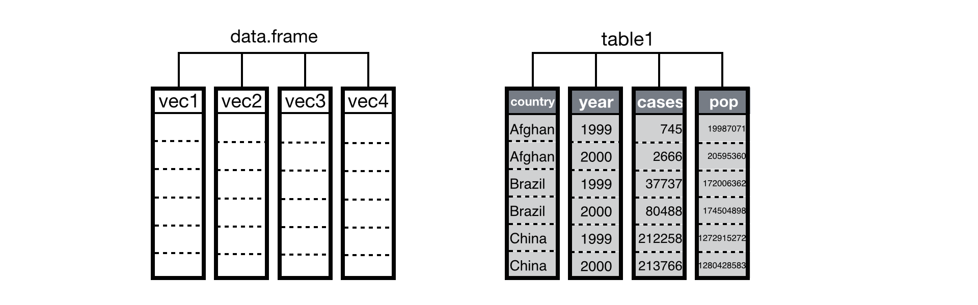
Data Frames

Data frames are used for storing Data tables in R. They are two-dimensional array structures and are similar to tables where each column represents one variable. The main features to note about a data frame are:

• Columns can be of different data types

• Each column name must be unique

• Each column should be of the same length i.e., contain the same number of elements

Data frames in R can be created in two ways:

• Using data.frame() command
• Importing data from files such as .csv, .xlsx etc.

data.frame() FUNCTION:

While using the command we can follow the below syntax

data. Frame (column_1, column_2, column_3, …………………….)

Make sure that the names of the columns are unique and are of the same length.

Creating a data frame

# input code

# Student ID, names and their marks.
student.data <- data.frame(
   std_id = c(001:005),
   std_name = c("William", "James", "Olivia", "Steve", "David"),
   std_marks = c(84.8, 98.4, 74.6, 80, 95)
)

# Display the dataframe student.data
student.data

# Check the structure of the dataframe student.data
str(student.data)

#check the head and tail of the dataframe student.data
head(student.data, 3)

tail(student.data, 3)


# Check the summary, lenth and dimension of the dataframe student.data
summary(student.data)

length(student.data)

dim(student.data)

# Check number of row/columns individually.
ncol(student.data)
nrow(student.data)

#output 
> # Student ID, names and their marks.
> student.data <- data.frame(
+    std_id = c(001:005),
+    std_name = c("William", "James", "Olivia", "Steve", "David"),
+    std_marks = c(84.8, 98.4, 74.6, 80, 95)
+ )
> 
> # Display the dataframe student.data
> student.data
  std_id std_name std_marks
1      1  William      84.8
2      2    James      98.4
3      3   Olivia      74.6
4      4    Steve      80.0
5      5    David      95.0
> 
> # Check the structure of the dataframe student.data
> str(student.data)
'data.frame':	5 obs. of  3 variables:
 $ std_id   : int  1 2 3 4 5
 $ std_name : chr  "William" "James" "Olivia" "Steve" ...
 $ std_marks: num  84.8 98.4 74.6 80 95
> 
> #check the head and tail of the dataframe student.data
> head(student.data, 3)
  std_id std_name std_marks
1      1  William      84.8
2      2    James      98.4
3      3   Olivia      74.6
> 
> tail(student.data, 3)
  std_id std_name std_marks
3      3   Olivia      74.6
4      4    Steve      80.0
5      5    David      95.0
> 
> 
> # Check the summary, lenth and dimension of the dataframe student.data
> summary(student.data)
     std_id    std_name           std_marks    
 Min.   :1   Length:5           Min.   :74.60  
 1st Qu.:2   Class :character   1st Qu.:80.00  
 Median :3   Mode  :character   Median :84.80  
 Mean   :3                      Mean   :86.56  
 3rd Qu.:4                      3rd Qu.:95.00  
 Max.   :5                      Max.   :98.40  
> 
> length(student.data)
[1] 3
> 
> dim(student.data)
[1] 5 3
> 
> # Check number of row/columns individually.
> ncol(student.data)
[1] 3
> nrow(student.data)
[1] 5

Accessing Dataframe

# input code

student.dataMaths <- data.frame(
  std_id = c(001:005),
  std_name = c("William", "James", "Olivia", "Steve", "David"),
  std_marks_maths = c(56.7, 60.8, 87.1, 55, 62.7)
)

# select columns
student.dataMaths[1]
student.dataMaths[-2]

#selecting columns ONLY data frames
# give the values as vector
student.dataMaths$std_marks_maths

#dataframe[Rows, Cols]

student.dataMaths[2]
student.dataMaths[2,]

student.dataMaths[c(1:3),]

# output
> student.dataMaths <- data.frame(
+    std_id = c(001:005),
+    std_name = c("William", "James", "Olivia", "Steve", "David"),
+    std_marks_maths = c(56.7, 60.8, 87.1, 55, 62.7)
+ )
> 
> # select columns
> student.dataMaths[1]
  std_id
1      1
2      2
3      3
4      4
5      5
> student.dataMaths[-2]
  std_id std_marks_maths
1      1            56.7
2      2            60.8
3      3            87.1
4      4            55.0
5      5            62.7
> 
> #selecting columns ONLY data frames
> # give the values as vector
> student.dataMaths$std_marks_maths
[1] 56.7 60.8 87.1 55.0 62.7
> 
> #dataframe[Rows, Cols]
> 
> student.dataMaths[2]
  std_name
1  William
2    James
3   Olivia
4    Steve
5    David
> student.dataMaths[2,]
  std_id std_name std_marks_maths
2      2    James            60.8
> 
> student.dataMaths[c(1:3),]
  std_id std_name std_marks_maths
1      1  William            56.7
2      2    James            60.8
3      3   Olivia            87.1

Data Transformation

#Input code 
student.dataEnglish <- data.frame(
   std_id = c(001:005),
   std_name = c("William", "James", "Olivia", "Steve", "David"),
   std_marks_eng = c(84.8, 98.4, 74.6, 80, 95)
)

student.marks <- data.frame(
   student.dataEnglish, 
   student.dataMaths[3])

student.marks

stud_6 <- data.frame(std_id = c(1:6))
stud_6

stud6_marks <- data.frame(
   student.dataEnglish, 
   stud_6)

student.dataEnglish

new_stdData <- data.frame(
   std_id = 006,
   std_name = "George",
   std_marks_eng = 75.6)

new_stdData

update.stdDataEng <- rbind(student.dataEnglish, new_stdData)

update.stdDataEng

# output
> student.dataEnglish <- data.frame(
+    std_id = c(001:005),
+    std_name = c("William", "James", "Olivia", "Steve", "David"),
+    std_marks_eng = c(84.8, 98.4, 74.6, 80, 95)
+ )
> 
> student.marks <- data.frame(
+    student.dataEnglish, 
+    student.dataMaths[3])
> 
> student.marks
  std_id std_name std_marks_eng std_marks_maths
1      1  William          84.8            56.7
2      2    James          98.4            60.8
3      3   Olivia          74.6            87.1
4      4    Steve          80.0            55.0
5      5    David          95.0            62.7
> 
> stud_6 <- data.frame(std_id = c(1:6))
> stud_6
  std_id
1      1
2      2
3      3
4      4
5      5
6      6
> 
> stud6_marks <- data.frame(
+    student.dataEnglish, 
+    stud_6)
Error in data.frame(student.dataEnglish, stud_6) : 
  arguments imply differing number of rows: 5, 6
> 
> student.dataEnglish
  std_id std_name std_marks_eng
1      1  William          84.8
2      2    James          98.4
3      3   Olivia          74.6
4      4    Steve          80.0
5      5    David          95.0
> 
> new_stdData <- data.frame(
+    std_id = 006,
+    std_name = "George",
+    std_marks_eng = 75.6)
> 
> new_stdData
  std_id std_name std_marks_eng
1      6   George          75.6
> 
> update.stdDataEng <- rbind(student.dataEnglish, new_stdData)
> 
> update.stdDataEng
  std_id std_name std_marks_eng
1      1  William          84.8
2      2    James          98.4
3      3   Olivia          74.6
4      4    Steve          80.0
5      5    David          95.0
6      6   George          75.6

Data Operations

# input code
# Create a dataframe for user data containing their
# IDs, Names, Age and heights in cm.
user.data <- data.frame(
   user.sn = c(1:5),
   user.name = c("Mr. A", "Mrs B", "Mrs. C", "Mr. D", "Mr. D"),
   user.age = c(25, 50, 41, 29, 58),
   user.height = c(181, 165, 155, 162, 142)
)
user.data
# Calculating sum of ages 
sum(user.data$user.age)

# Calculating the mean of user ages
mean(user.data[[3]])

# Calculating standard deviation of user ages
sd(user.data$user.age)

# Searching for 180 in user.data dataframe
"180" %in% user.data$user.height

"165" %in% user.data$user.height

# output
> # IDs, Names, Age and heights in cm.
> user.data <- data.frame(
+    user.sn = c(1:5),
+    user.name = c("Mr. A", "Mrs B", "Mrs. C", "Mr. D", "Mr. D"),
+    user.age = c(25, 50, 41, 29, 58),
+    user.height = c(181, 165, 155, 162, 142)
+ )
> user.data
  user.sn user.name user.age user.height
1       1     Mr. A       25         181
2       2     Mrs B       50         165
3       3    Mrs. C       41         155
4       4     Mr. D       29         162
5       5     Mr. D       58         142
> # Calculating sum of ages 
> sum(user.data$user.age)
[1] 203
> # Calculating the mean of user ages
> mean(user.data[[3]])
[1] 40.6
> # Calculating standard deviation of user ages
> sd(user.data$user.age)
[1] 13.86723
> 
> # Searching for 180 in user.data dataframe
> "180" %in% user.data$user.height
[1] FALSE
> 
> "165" %in% user.data$user.height
[1] TRUE

Key Points

• basic statistical knowledge and formulas

sample dataset and importing data in R studio

Overview

Time: min

Objectives

• learning how to use the sample dataset

• understanding how to import data in R studio

Sample Dataset

• One of the easiest ways to start experimenting with the analysis in R is by means of built-in sample datasets available in R. These datasets are available in their own package.

• Use the code provided in the script to load the dataset and then toggle through help function to know the complete information of the dataset.

# INSTALL AND LOAD PACKAGES ################################

# Load base packages manually
library(datasets) # For example datasets
?datasets
library(help = "datasets")

# SOME SAMPLE DATASETS #####################################

iris
?iris

cars <-cars

head(cars)

iris <- iris
head(iris)

tail(iris,20)

iris[,c(1,2)]

iris[,c('Sepal.Length')]


str(iris)

rm(list = ls())

iris

# CLEAN UP #################################################

# Clear environment
rm(list = ls()) 

# Clear packages
detach("package:datasets", unload = TRUE)  # For base

# Clear plots
dev.off()  # But only if there IS a plot

# Clear console
cat("\014")  # ctrl+L

Importing data

There are multiple commands with various arguments to import data from different file formats into R environment. I shall show the simplest command to import a csv file as a data frame

data_frame_name <- read.csv(file. choose(), header = T)

Here, file. choose() - Allows you to choose a .csv file stored in your local desktop

Here, header = T - Indicates the first row in the file contains column names.

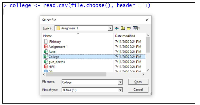
Double click (or) click once and select open on your desired file to import

Once the data has been imported successfully the data frame would be visible with its name in the Environment pane on the top right.

Packages

• One of the most important things in R is its collection of Packages. The package is a collection of R functions, data, and compiled code and Library is the location where the packages are stored. In order to access these packages, we can either go to r-project. Org > CRAN> 0 Cloud> packages>CRAN task view or use the command library() to load the package in the current R session.
• Then just call the appropriate package functions

install.packages(“package_name”) – Install the package from CRAN repository

install.packages( c(“package_1”, “”package_2”, “package_3”) ) -Install multiple packages

library(“package_name”) – Load the package in current R session.

# first step of using a package
install.packages("tidyverse")

# second step - needs happen each session
# load library
library(tidyverse)

## load data from elsewhere

df <- read_csv("data/StateData.csv")

Key Points