Scientific reproducibility: What is it for?
Overview
Time: 15 minObjectives
Understand what scientific reproducibility entails.
Identify the benefits of using RStudio to create research reports.
Understand how RStudio supports Open Science principles.
Learn how RStudio can help one’s research.
Warm-up
Let’s get into breakout rooms and discuss: What is reproducible research for you? Have you ever experienced issues while trying to reproduce someone else’s study or even your own research?
Reproducible studies allow other researchers to perform the same processes and analyses to produce an identical result as the first initial researcher. Original researchers have to make available the study’s associated data, documentation, and code pipelines and workflows in a way that is sufficiently self-explanatory and well-documented so that independent investigators can reproduce/recreate the original study under the same conditions, using identical materials and procedures, and ultimately achieve consistent results and render equal outcomes. Original investigators, therefore, must produce rich and detailed documentation for themselves and others. This includes fully specifying both in human-readable and computer-executable ways all steps taken in the study.
The importance of Reproducibility in Research
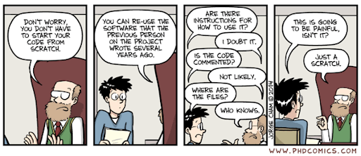
Source: Comic number 1869 from PhD Comics Copyrighted artwork by Jorge Cham.
Discussion: A scary anecdote
- A group of researchers obtain great results and submit their work to a high-profile journal.
- Reviewers ask for new figures and additional analysis.
- The researchers start working on revisions and generate modified figures, but find inconsistencies with old figures.
- The researchers can’t find some of the data they used to generate the original results, and can’t figure out which parameters they used when running their analyses.
- The manuscript is still languishing in the drawer…
According to the U.S. National Science Foundation (NSF)subcommittee on replicability in science (2015):
Science should routinely evaluate the reproducibility of findings that enjoy a prominent role in the published literature. To make reproduction possible, efficient, and informative, researchers should sufficiently document the details of the procedures used to collect data, to convert observations into analyzable data, and to perform data analysis.
Reproducibility refers to the ability of a researcher to duplicate the results of a prior study using the same materials as were used by the original investigator. That is, a second researcher might use the same raw data to build the same analysis files and implement the same statistical analysis in an attempt to yield the same results. Reproducibility is a minimum necessary condition for a finding to be considered rigorous, believable and informative.
Why all the talk about reproducible research?
A 2016 survey in Nature revealed that irreproducible experiments are a problem across all domains of science:
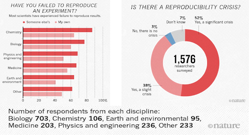
Source: Baker, M. 1,500 scientists lift the lid on reproducibility. Nature 533, 452–454 (2016). doi.org/10.1038/533452a
Factors behind irreproducible research

Source: Then a Miracle Occurs. Copyrighted artwork by Sydney Harris Inc.
- Not enough documentation on how experiment is conducted and data is generated
- Data used to generate original results unavailable
- Software used to generate original results unavailable
- Difficult to recreate software environment (libraries, versions) used to generate original results
- Difficult to rerun the computational steps
Reproducible, replicable, robust, generalizable
While reproducibility is the minimum requirement and can be solved with “good enough” computational practices, replicability/robustness/generalizability of scientific findings are an even greater concern involving research misconduct, questionable research practices (p-hacking, HARKing, cherry-picking), sloppy methods, and other conscious and unconscious biases.
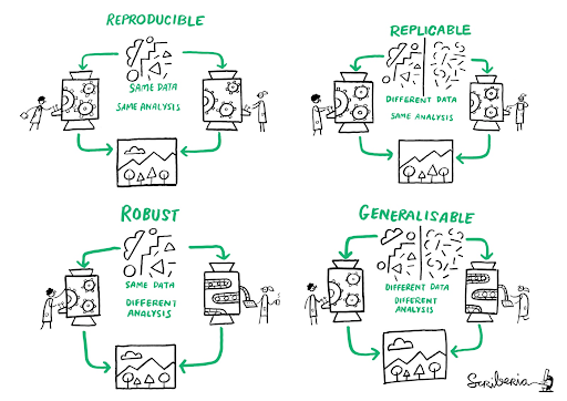
Source: This image was created by Scriberia for The Turing Way community DOI: 10.5281/zenodo.3 332807
If contributing to science and other researchers seems not to be compelling enough, here are 5 selfish reasons to work reproducibly according to Markowetz (2015):
- Helps to avoid data loss and disaster
- Makes it easier to write papers
- Helps reviewers see it your way
- Enables continuity of your work
- Helps to build your reputation
When do you need to worry about reproducibility?
Let’s assume that I have convinced you that reproducibility and transparency are in your own best interest. Then what is the best time to worry about it?
From day one, and throughout the whole research life cycle! Before you start the project because you might have to learn tools like R or Git. While you do the analysis because if you wait too long you might lose a lot of time trying to remember what you did two months ago. When you write the paper because you want your numbers, tables, and figures to be up-to-date. When you co-author a paper, because you want to make sure that the analyses presented in a paper with your name on are sound. When you review a paper, because you can’t judge the results if you don’t know how the authors got there.
Levels of Reproducibility
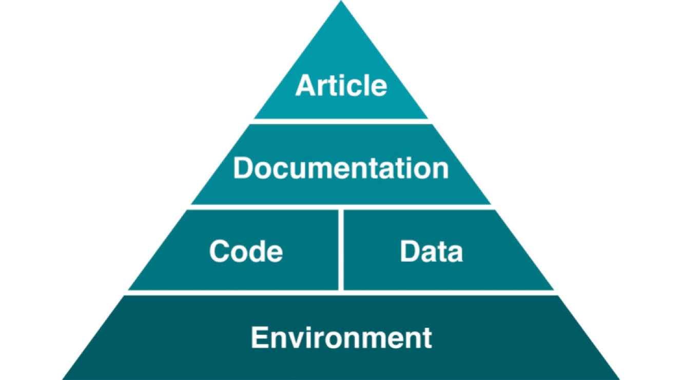
A published article is like the top of a pyramid, meaning that a reproducible paper/report rests on multiple levels that each contributes to its reproducibility.
Advantages of using RStudio for your project
RStudio is an integrated development environment (IDE) for R. It includes a console, syntax-highlighting editor that supports direct code execution, as well as tools for plotting, history, debugging, collaboration, and workspace management.
Creates documents using R Markdown
R Markdown is a variant of Markdown, a system for writing simple, readable text that is easily converted to html which allows you to write using an easy-to-read, easy-to-write plain text format.
R Markdown belongs to the field of literate programming which is about weaving text and source code into a single document to make it easy to create reproducible web-based reports. Markdown is a simple formatting syntax for authoring HTML, PDF, and MS Word documents and much, much more. R Markdown provides the flexibility of Markdown with the implementation of R input and output. For more details on using R Markdown check http://rmarkdown.rstudio.com.
The idea of literate programming shines some light on this dark area of science. This is an idea from Donald Knuth where you combine your text with your code output to create a document. This is a blend of your literature (text), and your programming (code), to create something that you can read from top to bottom. Imagine your paper - the introduction, methods, results, discussion, and conclusion, and all the bits of code that make each section. With R Markdown, you can see all the pieces of your data analysis altogether.
You can include both text and code to execute. It is a convenient tool for reproducible and dynamic reports with R! With R Markdown, you are able to:
- Keep an eye on text (the paper) AND the source code. These computational steps are essential to ensure computational reproducibility.
- Conduct the entire analysis pipeline in an R Markdown document: data (pre-)processing, analysis, outputs, visualization.
- Apply a formatting syntax that is part of the R ecosystem and supports LaTeX.
- Combine text written in Markdown and source code written in R (and other languages).
- Easily share R Markdown documents with colleagues, as supplemental material, or as the paper under review. Thanks to the package knitr, others can execute the document with a single click and receive, for example, HTML or PDF renderings.
- Get figures automatically updated if you change the underlying parameters in the code. The error-prone task of exporting figures and uploading the right figure version to another platform is thus not needed anymore.
- Since Markdown is a text-based format, you can also use versioning control with Git.
- If you do not make any changes to the document after creating the output document, you can be sure that the paper was executable at least at the time of submission.
- Refer to the corresponding code lines in the methodology section making it unnecessary to use pseudocode, high-level textual descriptions, or just too many words to describe the computational analysis.
- Use packages such as rticles to use templates from publishers and create submission-ready documents.
Integrates with Collaboration and Publishing Tools
Another great advantage of using Rstudio for your R project is that the platform integrates with GitHub. Once you connect RStudio with your GitHub account a remote repo becomes the “upstream” remote for your local repo. In essence, it enables you push and pull commits to GitHub allowing more seamless collaboration and more effective version control. RStudio also connects with Rpubs for easy R project web publishing.
Some Real-world Applications
Finally, three real-world examples that motivated the authors of this lesson to value and use R Markdown:
-
Greg Janee quickly put together a simple but compelling R Markdown document describing his survey results. The ease with which he created his plots is a testament to the power of R as a data analysis environment, but the ease with which he was able to publish a page on the web is a testament to R Markdown and Github as a publishing environment. Notice that he did not have to: create plots in a tool and then export the plots as images; write any HTML; embed plot images in HTML; or create a site under Wordpress or other web hosting service. Instead, he directly published his R code as he wrote it, and using GitHub, made it appear on the web with a button click.
-
One of us wanted to create a short document that included some math formulas. The LaTeX document preparation can be used for this, but it is difficult to use and is overkill for just a few formulas in otherwise plain text. R Markdown lets you use just the best part of LaTeX—math formatting—while letting you write your text in a user-friendly way.
-
In this lesson we will be constructing a scientific paper that is based on an actual Nature publication and attendant survey and data. In trying to recreate the plots the original authors created, we found it difficult and time-consuming to figure out exactly how the authors created their plots. Out of the many columns in their data, many with similar-sounding names, which did they use? How did they handle missing data? Exactly what operations did they perform to compute aggregate values? How much easier it would have been if they had published the code they used along with their paper. R Markdown allows you to do this.
Our goal is that by the end of this workshop you will be able to create a reproducible report. This template is a short and adapted version of the data paper referenced below:
Nitsch, F. J., Sellitto, M., & Kalenscher, T. (2021). Trier social stress test and food-choice: Behavioral, self-report & hormonal data. Data in brief, 37, 107245. https://doi.org/10.1016/j.dib.2021.107245
This template is used exclusively for instruction purposes with permission from the authors.
Key Points
Reproducible research is key for scientific advancement.
RStudio can help you to organize, have better control over and produce reproducible research.
Navigating RStudio and R Markdown Documents
Overview
Time: 20 minObjectives
Understand key functions in Rstudio.
Learn about the structure of a Rmarkdown file.
Understand the workflow of an R Markdown file.
Getting Around RStudio
Throughout this lesson, we’re going to teach you some of the fundamentals of using R Markdown as part of your RStudio workflow.
We’ll be using RStudio: a free, open source R Integrated Development Environment (IDE). It provides a built in editor, works on all platforms (including on servers) and provides many advantages such as integration with version control and project management.
This lesson assumes you already have a basic understanding of R and RStudio but we will do a brief tour of the IDE, review R projects and the best practices for organizing your work, and how to install packages you may want to use to work with R Markdown.
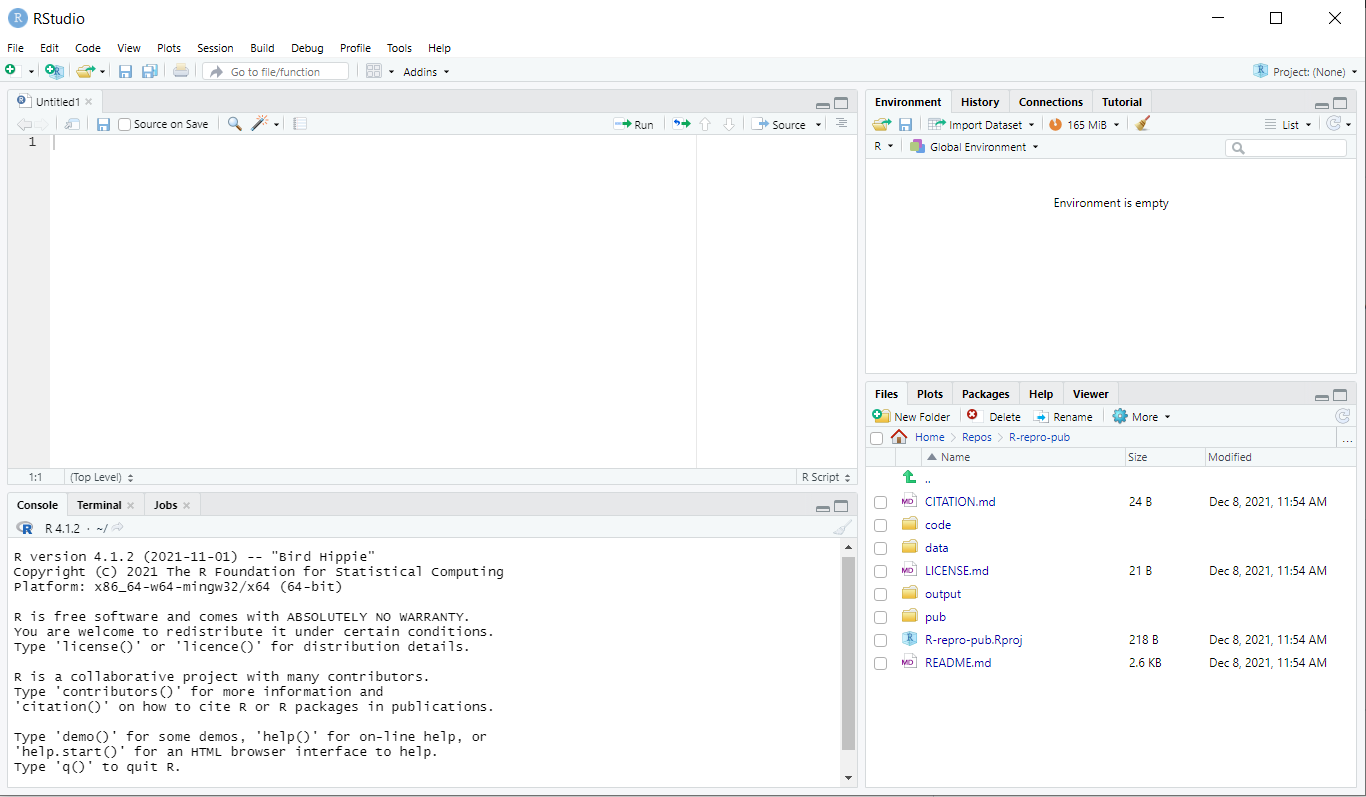
Basic layout
When you first open RStudio, you will be greeted by three panels:
- The interactive R console/Terminal (entire left)
- Environment/History/Connections (tabbed in upper right)
- Files/Plots/Packages/Help/Viewer (tabbed in lower right)
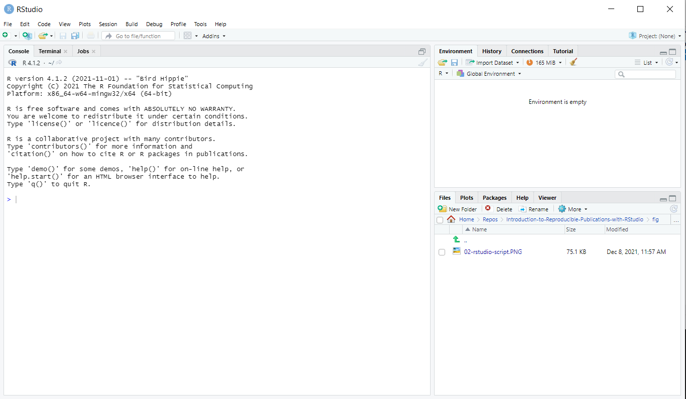
Once you open files, such as .Rmd files or .R files, an editor panel will also open in the top left.
R Packages
It is possible to add functions to R by writing a package, or by obtaining a package written by someone else. As of this writing, there are over 10,000 packages available on CRAN (the comprehensive R archive network). R and RStudio have functionality for managing packages:
- You can see what packages are installed by typing
installed.packages() - You can install packages by typing
install.packages("packagename"), wherepackagenameis the package name, in quotes. - You can update installed packages by typing
update.packages() - You can remove a package with
remove.packages("packagename") - You can make a package available for use with
library(packagename)
Packages can also be viewed, loaded, and detached in the Packages tab of the lower right panel in RStudio. Clicking on this tab will display all of installed packages with a checkbox next to them. If the box next to a package name is checked, the package is loaded and if it is empty, the package is not loaded. Click an empty box to load that package and click a checked box to detach that package.
Packages can be installed and updated from the Package tab with the Install and Update buttons at the top of the tab.
CHALLENGE 2.1 - Installing Packages
Install the following packages:
bookdown,tidyverse,knitr,rticles,BayesFactor,patchwork,rprojrootSOLUTION
We can use the
install.packages()command to install the required packages:install.packages("bookdown") install.packages("tidyverse") install.packages("knitr") install.packages("rticles") install.packages("BayesFactor") install.packages("patchwork") install.packages("rprojroot")An alternate solution, to install multiple packages with a single
install.packages()command is:install.packages(c("bookdown", "tidyverse", "knitr", "rticles", "BayesFactor", "patchwork", "rprojroot"))
Starting a R Markdown File
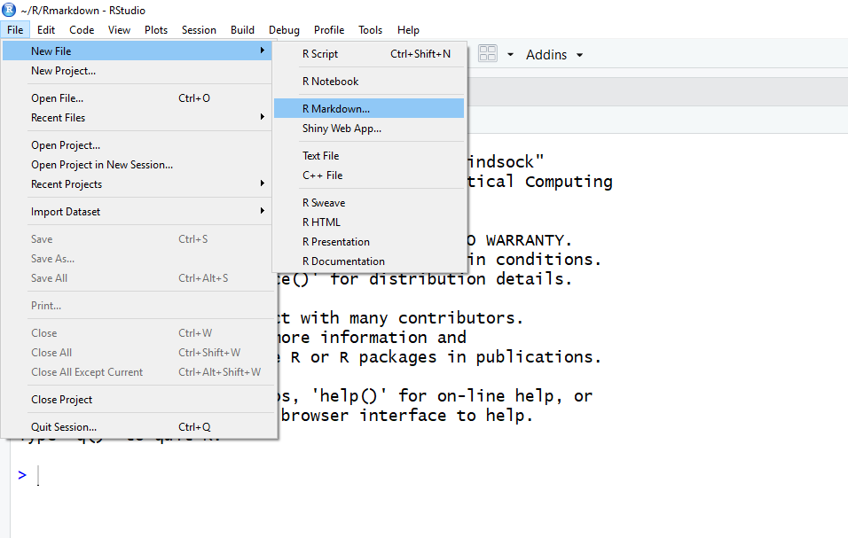
Start a new R Markdown document in RStudio by clicking File > New File > R Markdown…
If this is the first time you have ever opened an R Markdown file a dialog box will open up to tell you what packages need to be installed. You shouldn’t see the dialog box if you installed these packages before the workshop.
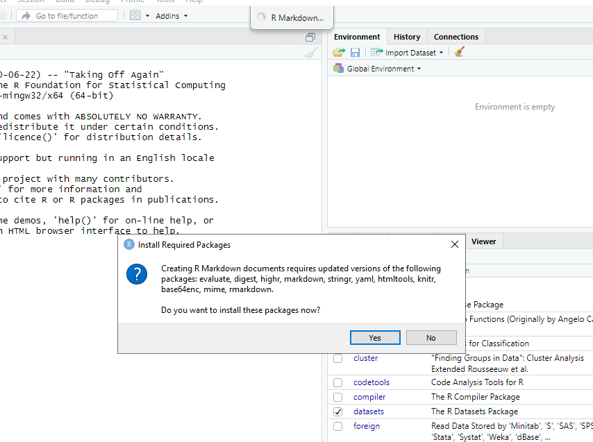
Click “Yes”. The packages will take a few seconds (to a few minutes) to install. You should see that each package was installed successfully in the dialog box.
Once the package installs have completed, a dialog box will pop up and ask you to name the file and add an author name (may already know what your name is) The default output is HTML and as the wizard indicates, it is the best way to start and in your final version or later versions you have the option of changing to pdf or word document (among many other output formats! We’ll see this later).
Naming your new R Markdown Document
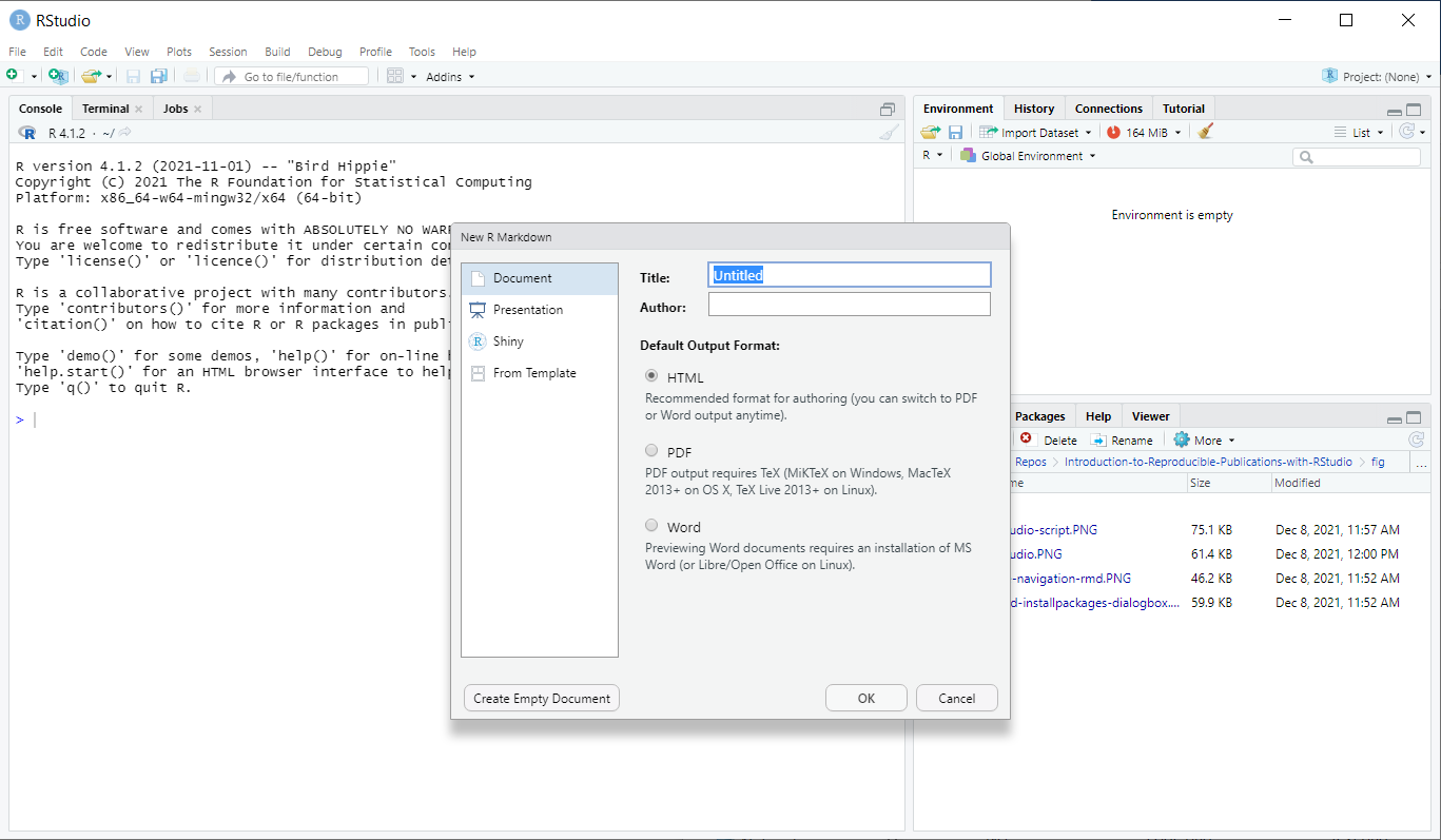
New R Markdown files will have a generic template unless you click the “Create Empty Document” in the bottom left-hand corner of the dialog box.
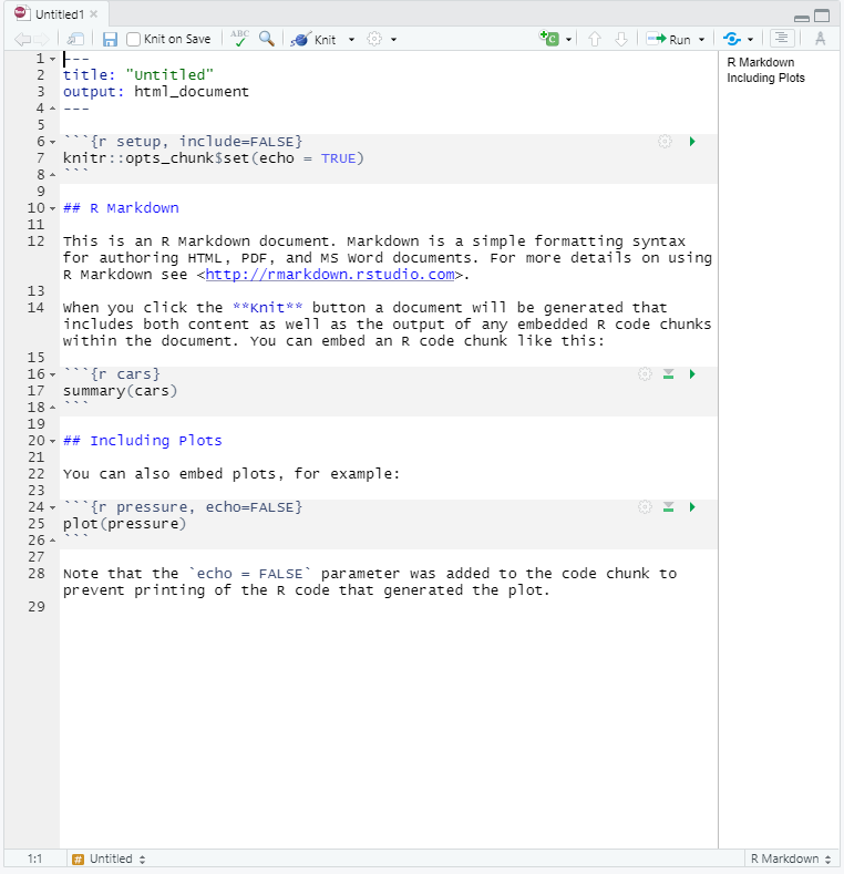
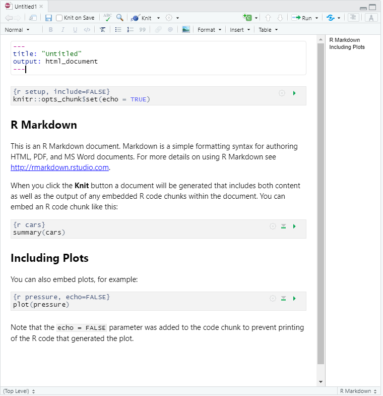
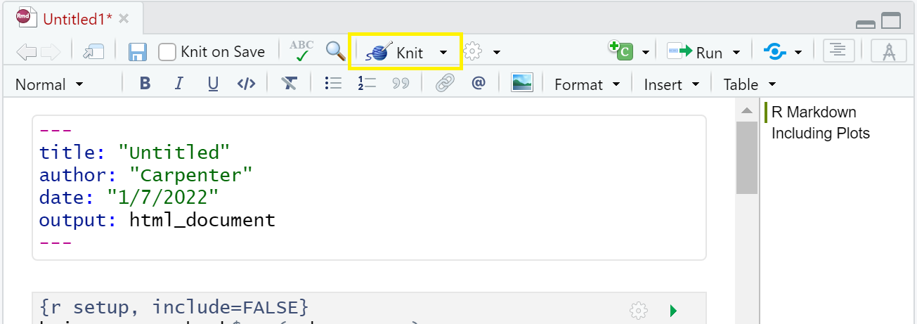
If you see this default text you’re good to go: 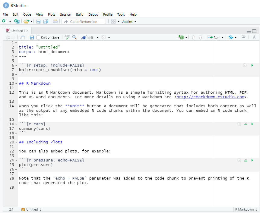
Visual Editor vs. Source Editor
RStudio released a new major update to their IDE in January 2020, which includes a new “visual editor” for R Markdown to supplement their original editor (which we will call the source editor) for authoring with R Markdown syntax. The new visual editor is friendlier with a graphical user interface similar to Word or Google docs that lets you choose styling options from the menu (before you had to either have the R Markdown code memorized or look it up for each of your styling choices). Another major benefit is that the new editor renders the R Markdown styling in real time so you can preview your paper before rendering to your output format.
Source Editor
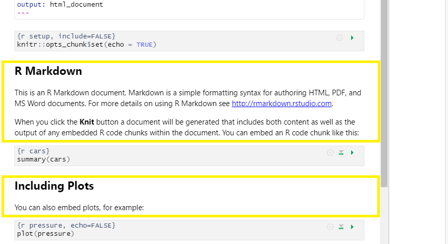
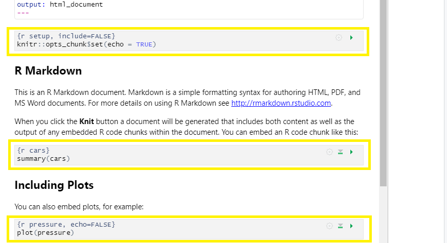
The image below displays the default R Markdown template in the “source editor” mode. Notice the symbols scattered throughout the text (#, *, <>). Those are examples of R Markdown syntax, which is a flavor of Markdown syntax, an easy and quick, human-readable markup language for document styling.
CHALLENGE 2.2 - Formatting with Symbols (optional)
In Rmd certain symbols are used to denote formatting that should happen to the text (after we “knit” or render). Before we knit, these symbols will show up seemingly “randomly” throughout the text and don’t contribute to the narrative in a logical way. In the template Rmd document, there are three types of such symbols (##, **, <>) . Each symbol represents a different kind of formatting (think of your text formatting buttons you use in Word). Can you deduce from the surrounding text how these symbols format the surrounding text?
## R Markdown

This is an R Markdown document. Markdown is a simple formatting syntax for authoring HTML, PDF, and MS Word documents. For more details on using R Markdown see <http://rmarkdown.rstudio.com>.

When you click the **Knit** button a document will be generated that includes both content as well as the output of any embedded R code chunks within the document. You can embed an R code chunk like this:
SOLUTION
##is a heading,**is to bold enclosed text, and<>is for hyperlinks. Don’t worry about this too much right now! This is an example of R Markdown syntax for styling, you won’t need it if you stick to the visual editor, but it is recommended to get at least a basic understanding of R Markdown syntax if you plan to work with.rmddocuments frequently.
Switch to the visual editor
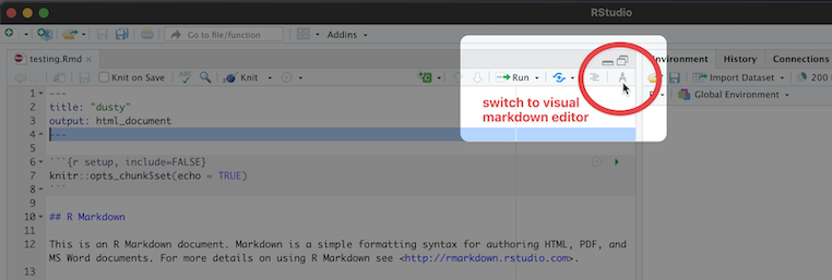
The new visual editor is accessible through a small button on the far right side of the script/document pane in RStudio. The icon is a protractor, but from further away it just looks like a squiggly “A”. See the image below to find the visual editor button, it isn’t the most obvious!
Visual Editor
We’ve already touched on the visual editor and it’s useful features, but now that we’ve switched to the visual editor take another look at your document and see what’s changed. You’ll notice that formatting elements like headings, hyperlinks and bold have been generated automatically, giving us a preview of how our text will render. However, the visual editor does not run any code automatically, we’ll have to do that manually (but we will learn how to do that later on).
We will proceed using the visual editor during this workshop as it is more user-friendly and allows us to talk about styling without needing to teach the whole R Markdown syntax system. However, we highly encourage you to become familiar with markdown syntax (specifically the R Markdown flavor) as it increases your abilities to format and style your paper without relying on the visual editor options.
Tip: Resources to learn R Markdown
if you want to learn how to use the source editor (as we call it) please see the the Pandoc Markdown Documentation. You will need to know Markdown formatting (specifically R-flavored Markdown).
Now we’ll get into how our R Markdown file & workflow is organized and then on to editing and styling!
Key Points
RStudio has 4 panes to organize your code and environment.
Install packages in RStudio using the
install.packages()function.R Markdown documents combine text and code.
Introduction to Working with R Markdown Files
Overview
Time: 20 minObjectives
Learn about the structure of a R Markdown file.
Learn how an R Markdown file works.
Learn how to knit/render a rmd file into an output format.
Understand what templates are and the advantage of using them.
Learn how to start a document from a template.
Anatomy of an R Markdown File
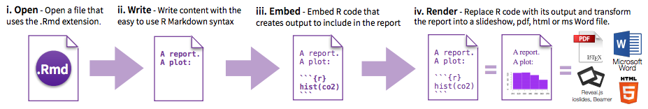
The key to our reproducible workflow is using R Markdown files in RStudio rather than basic scripts to dynamically “knit” both code and paper narrative. So let’s do a quick anatomy lesson on the components of an R Markdown file (YAML header, R Markdown formatted, R code chunks) and how to render them into our final formatted document. There are four distinct steps in the R Markdown workflow:
- create a YAML header (optional)
- write R Markdown-formatted text
- add R code chunks for embedded analysis
- render the document with Knitr
Let’s dig in to those more:
1. YAML header:
What is YAML anyway?
YAML, pronounced “Yeah-mul” stands for “YAML Ain’t Markup Language”. YAML is a human-readable data-serialization language which, as its name suggests, is not a markup language. YAML has no executable commands though it is compatible with all programming languages and virtually any application that deals with storing or transmiting data. YAML itself is made up of bits of many languages including Perl, MIME, C, & HTML. YAML is also a superset of JSON. When used as a stand-alone file the file ending is .yml or .yaml.
R Markdown’s default YAML header includes the following metadata surrounded by three dashes ---:
- title
- author
- date
- output
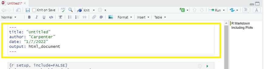
The first three are self-explanatory, but what’s the output? We saw this in the wizard for starting a new document, by default you are able to pick from pdf, html, and word document. Basically, this allows you to export your rmd file as a file type of your choice. There are other options for output and even more can be added by installing certain packages, but these are the three default options.
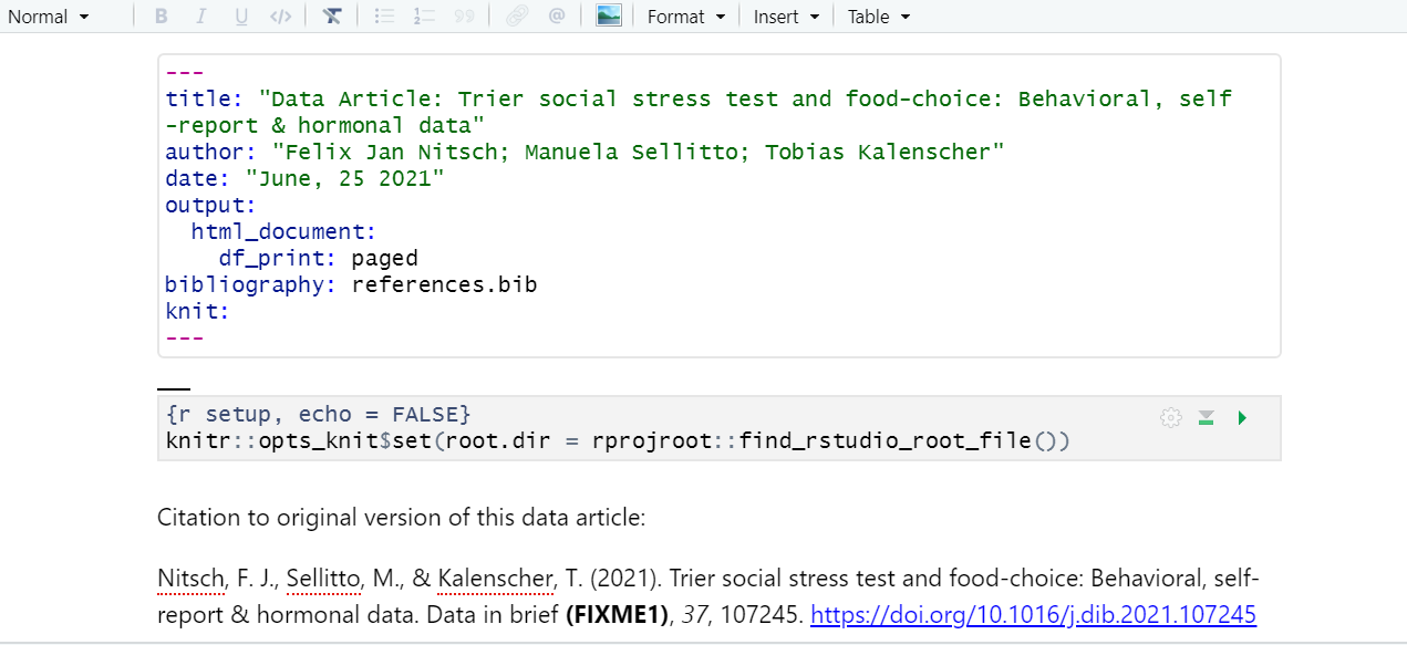
We’ll see other formatting options for YAML later on including how to add bibliography information, customize our output, and change the default settings of the knit function. Below is an example of how our YAML file will look at the end of this workshop.
---
---
title: "Data Article: Trier social stress test and food-choice: Behavioral, self-report & hormonal data"
author: "Felix Jan Nitsch; Manuela Sellitto; Tobias Kalenscher"
date: "June, 25 2021"
output:
  html_document:
    df_print: paged
bibliography: references.bib
knit: (function(rmdFile, encoding) {
      out_dir <- '../output';
      rmarkdown::render(rmdFile,
                        encoding=encoding,
                        output_file=file.path(dirname(rmdFile),
                        out_dir,
                        'DataPaper-ReproducibilityWorkshop.html'))})
---
---
2. Formatted text:
This one is simple, it’s literally just text narrative formatted by using markdown (more on markdown syntax later). Markdown-formatted text is one of the benefits added above and beyond the capabilities of a regular r script. Any text section will have the default white background in the rmd document. As you might know, in a regular R file, # starts a comment. In R markdown, plain text is just plain narrative text that appears in the document. In R scripts, plain text wants to be code. In R Markdown, you will need to enclose your code in special characters. Any symbols you do see that aren’t regular grammar components are for formatting, such as ##, ** **, and < >.
Tip: Bonus! You can use a variety of languages to format text and images in R Markdown:
- R Markdown
- HTML
- LaTeX
- CSS
3. Code Chunks:
R code chunks appear highlighted in gray throughout the rmd document. They are surrounded by three tick marks on either side (```) in source mode with the starting three tick marks followed by curly brackets {}with some other code inside. The tick marks indicate the start of a code section and the bits found between the curly brackets {}indicate how R should read and display the code (more on this in the Knitr syntax episodes). These are the sections you add R code such as summary statistics, analysis, tables and plots. If you’ve already written an R script you can copy and paste your code between the few lines of required formatting to embed & run whichever piece you want at that particular spot in the document.
Tip: Bonus! You may code with many different languages in RStudio:
- R
- Python
- Bash
- SQL
A complete list of compatible languages can be found at: https://rmarkdown.rstudio.com/lesson-5.html
4. Rendering your Rmd document:
This is called “knitting” and the button looks like a spool of yarn with a knitting needle. Clicking the knit button will compile the code, check for errors, and finally, output the type of file indicated in your yaml header. One nice thing about the knit button is that it saves the .Rmd document each time you run it. Your rmd document may not run and render as your indicated output if there are any errors in the document so it also functions somewhat as a code checker.
Try it yourself
We’re going to pause here and see what the R Markdown does when it’s rendered. We’ll just use the generic template, but when we’re working on our own project, knitting periodically while we’re editing allows us to catch errors early. We’ll continue rendering our rmd throughout the lesson to see what happens when we add our markdown and knitr syntax and to make sure we aren’t making any errors.
This is a little preview of what’s to come in the later episodes: Click the “knit” button.
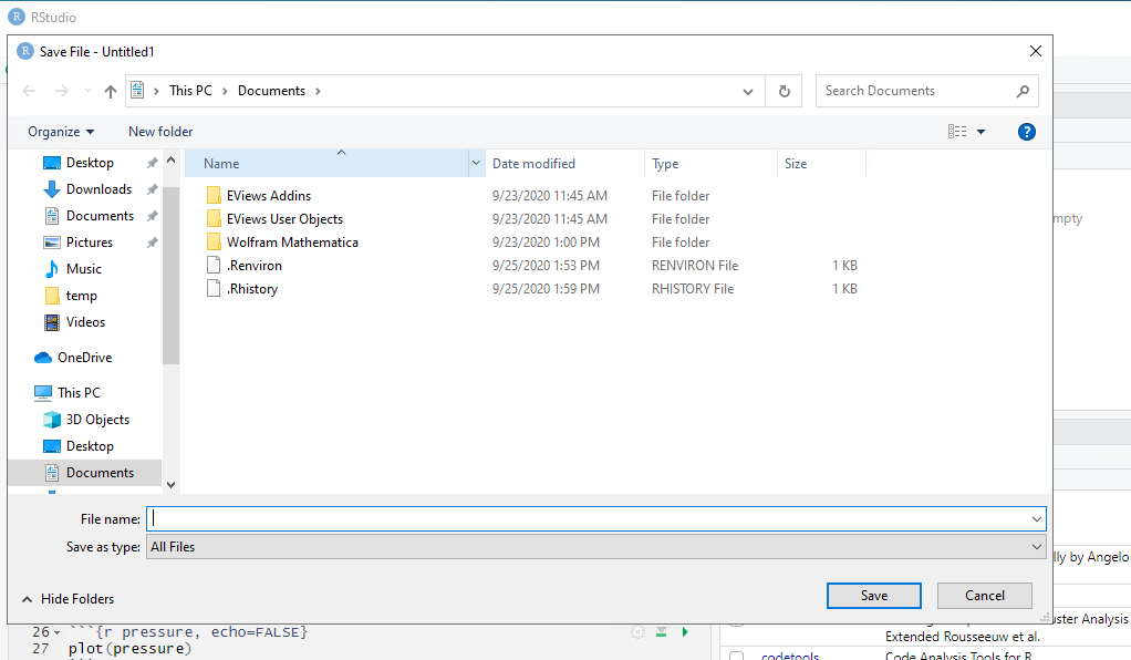
Before you can render your document, you’ll need to give it a file name and choose what folder you want to save it to. Choose my_first_rmd.rmd as your file name and save it to an easily accessible directory in your file system.
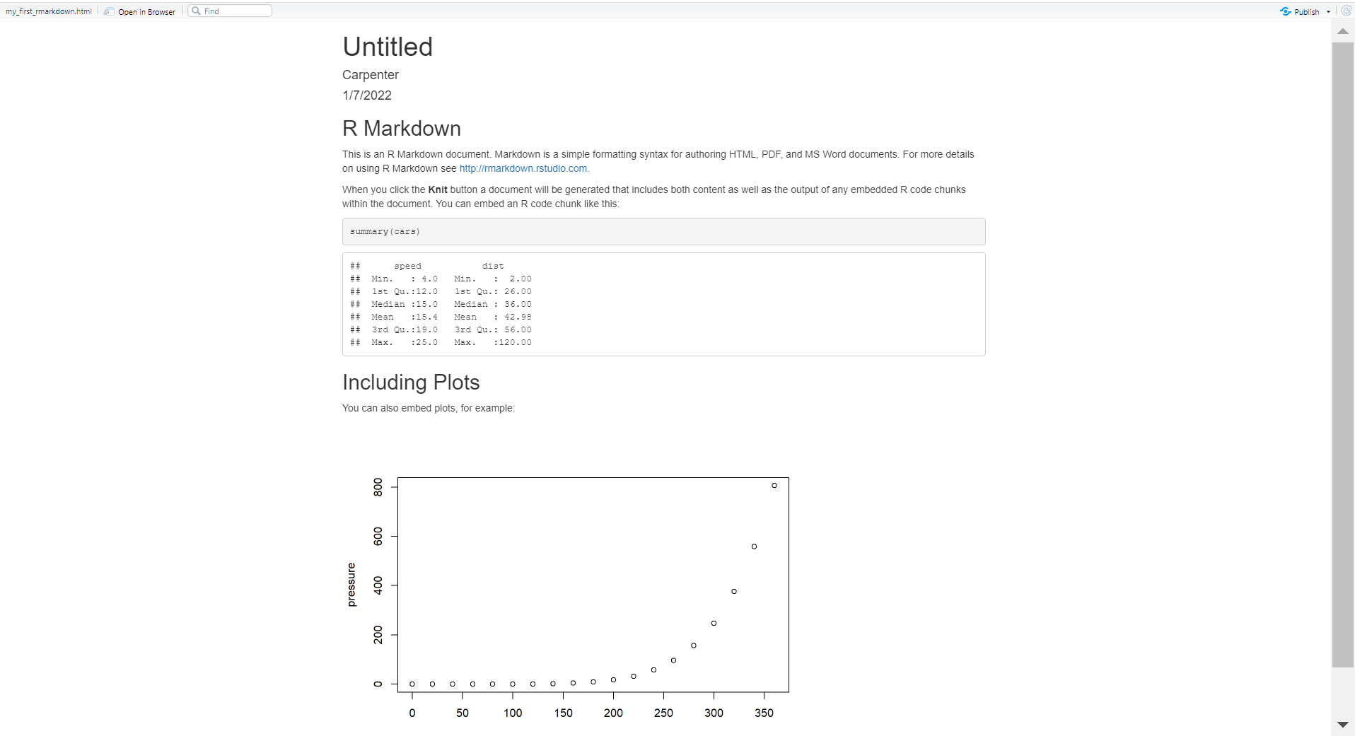
This is how our html document will render after clicking the knit button and choosing a file name:
CHALLENGE 3.1 - Rendering the document in another format
Suppose you want this .rmd document to render as a word document. What options would you have?
Solution:
1) You may change the output format in the YAML to
word_document, or 2) Select “Knit > “Knit to Word” on the menu.
Finding and Applying Existing Templates
We have learned how to start a new document on RStudio and we will learn good practices for project organization next. But, let’s say you are writing a paper and you already know which journal you are submitting it to? Writing it in your own style and then formatting prior to submission is time-consuming, right? The good news is that RStudio makes our lives easier. Through a package called “rticles” you can access a number of existing journals’ templates that will let you easily and quickly format and prepare your paper draft for peer review. Even if the journal you submit to does not have a template, it may be good to review several of the templates to get an idea of formatting options available to you in R Markdown..
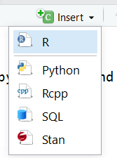
Let’s take a look at that! On RStudio, load the rticles package by using the function library(rticles) (remember we’ve already installed the package earlier!). Once you’ve loaded the package, use the plus icon at the upper-left side of your screen to create a new document or proceed with File > New File > R Markdown. This will prompt the window for creating a new R Markdown document as we saw earlier.
Clicking on “From Template” will prompt a couple of dozen templates listed as {rticles}. Let’s choose the Biometrics Journal template and then, OK.
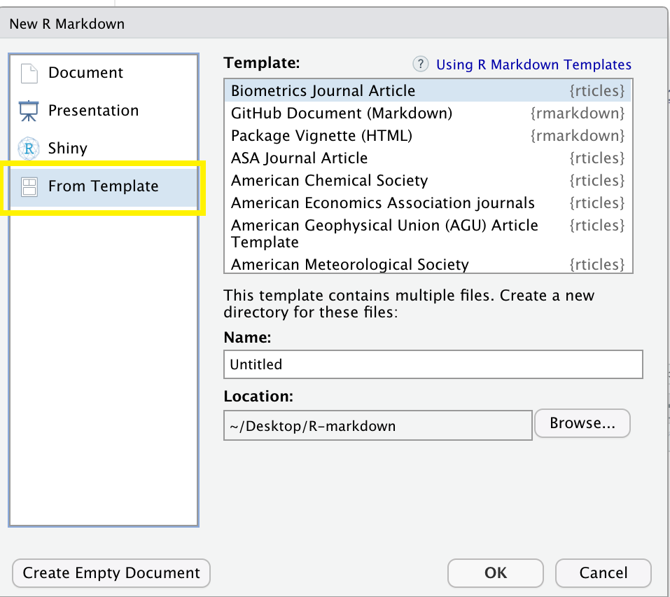
Note that along with the skeleton of the paper you will see a message on top indicating additional packages you may need to install for that particular template.
Tip: Create your own template
Please remember that for this workshop we are producing a report in html and not tied to a particular journal template. You may choose other output formats such as word or pdf. Creating templates and adding other templates is beyond the scope of this workshop, but that is also possible. If you submit to the same journal frequently or use the same formatting for many of your publications, it may be worth creating your own template to save time. To learn more about how you can create templates in RStudio:
- Using R Markdown Templates on the right-hand side check the rticles package documentation
- How to contribute to a new article template?
Challenge: Find a template (optional):
Find the template for the Bioinformatics Journal, what does the template look like? What sections does it contain?
Discussion: What may be the pros and cons of using an existing template? (optional)
Solution:
Pros:
- Formatting papers according to journals’ guidelines can be very cumbersome and time-consuming. So, using a template for a specific journal will save you time!
Cons:
- If, along the way, you change your mind about the journal you were planning to submit to, there is no easy conversion to another template. Overwritting will cause problems.
- There are only a few journal titles available.
Tips:
- Always check if the template meets the most updated guidelines in the journal website. Since the rticles package is maintained by a community, we advise you check their (GitHub page][https://github.com/rstudio/rticles) for more details.
- Did not find a particular template? You can recommend one to the community or become a contributor!
Key Points
An R Markdown file is comprised of a YAML header, formatted text in rmd and code chunks.
The knit function renders the file into the chosen output format.
Rstudio has some journals’ templates that can save you some formatting time or you can make your own for frequent submissions.
Writing and Styling Rmd Documents
Overview
Time: 10 minObjectives
Learn how to enable the visual editor.
Get familiar with its basic functionalities.
Apply rmd formatting and styling using the visual editor.
Learn how to add inline code to your rdm document.
Formatting Rmd Documents with the Visual Editor
As we mentioned earlier, the visual editor in RStudio has made R Markdown formatting much more effortless. It provides improved productivity for composing longer-form articles and analyses with R Markdown. The visual markdown editing is available in RStudio v1.4 or higher. Markdown documents can be edited in either source or visual mode. To switch into visual mode for a given document, toggle on the compass icon at the top-right of the document toolbar (alternatively for windows, the ⌘⇧ F4 keyboard shortcut). This will prompt a formatting bar through which you can apply styling, add links, create tables, and others similar to functions you find in google docs and other document editors. Note that you can switch between source and visual mode at any time (editing location and undo/redo state will be preserved when you switch). Let’s try it! Feel free to follow along or just watch this quick demo. But first, make sure to have your visual editor enabled on your screen. Also, make sure to open your DataPaper-ReproducibilityWorkshop.Rmd file located at the report\source folder
Editor Toolbar
The editor toolbar includes buttons for the most commonly used formatting commands:

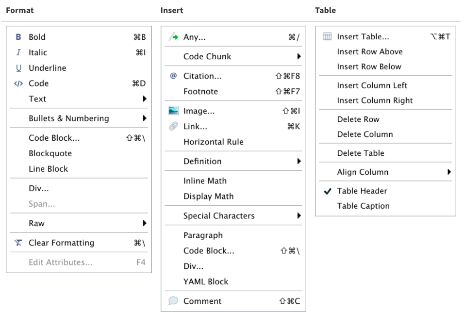
Additional commands are available on the Format, Insert, and Table menus:
Tip: Inserting anything with shortcuts
You can also use the catch-all ⌘ / shortcut to insert just about anything. Just execute the shortcut then type what you want to insert. For example:
/liswill prompt listing options.
Applying Emphasis
At the very top of the document we have a recommended citation for the sample data paper (FIXME1). We want to emphasize the title of the journal, “Data in brief” in italics. Select the text and click in the I icon and voilà! Remember to delete (FIXME1).
Adding Links
In the same citation we have just worked on, let’s now add a link to it by selecting and copying the doi address (FIXME2). Then, click on the link icon and paste the address in the URL field. Simple right? If you prefer, you can also the drop-down insert menu, or even use shortcuts. By hovering the mouse over the desired icon, you will see which keys you should use. For a complete list of editing shortcuts, check this link. Tip: if you didn’t intend to use a shortcut and want to reverse its effect, just press the backspace key.
Adding Headings
Adding headings to a R Markdown document in Rstudio is as simple as applying links. Let’s say we want the abstract section as a Heading Level 2. We can select the “abstract” then, and under “Normal” on the left-hand side of the menu, we can choose the desired level. Again, all the shortcuts will be listed next to the styling in the menu. Now apply the same heading to keywords and Level 2 to “Specification Table” (FIXME3).
Creating Tables
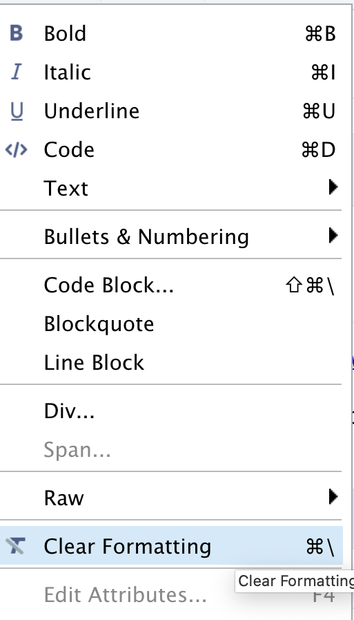
Because creating tables manually in Rmd documents could be a little painful for beginners, Rstudio released an add-in functionality for tables back in 2018. The new visual editor, however, have made the process to create rmd tables more similar to other editors we use daily. In our template, we have the specification table with 10 rows and two columns. If we were willing to add that table, we could do that by inserting a table to a selected part of the documents and by specifying the desired number of rows and columns. Including a caption is optional, but recommended. We can add or delete rows and columns, add a header that will be set bold by default but can be changed, and set the desired alignment. Select the desired text and click on the crossed T icon if you wish to clear formatting.
Creating Bullet and Numbered Lists
Again, similarly to other document editors, Rstudio allows you to turn text into bullet or numbered lists. Let’s apply a bullet list to the paragraphs specifying the “Values of the Data” reported in the data paper (FIXME4). Assuming we were willing to create a numbered list instead, we could have followed the same process and chosen the other icon. We can also sink or lift the listed items.
Adding Images
You may need to include static images to your manuscripts. For that, you can use the insert image function, click on the painting icon or even use the shortcut that shows right next to the function in the menu. After browsing and upload the desired image you may also specify the caption and the image title, as well as adjust dimensions if needed. Let’s insert two images Fig. 1 (FIXME5) and Fig. 2 (FIXME6).
Adding Formulas
If you have math formula in your manuscript there are three different ways you may insert one. Let’s look for (FIXME7) for an example. Point and click at the insert menu, use the catch-all ⌘ / keyboard short and then get to inline math mode, or type the formula content between dollar signs $. You will notice that the color and font type will change, as Rstudio identifies the block as an inline equation.
Keyboard Shortcuts
As you become a more regular Rstudio user, you may also consider using some keyboard shortcuts for all basic editing tasks. Visual mode supports both traditional keyboard shortcuts (e.g. ⌘ B for bold) as well as markdown shortcuts (using markdown syntax directly). For example, enclose bold text in asterisks or type ## and press space to create a second level heading. Here are some of the most commonly used shortcuts for Mac users:
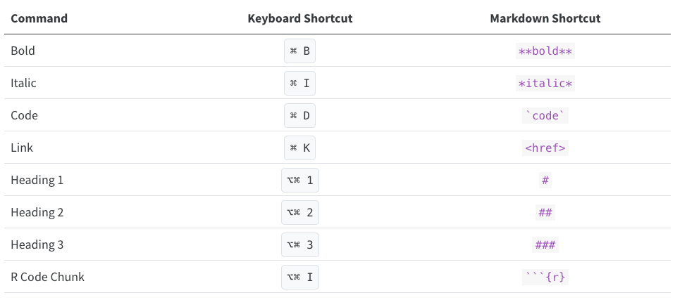
Tip: Windows users should replace in the shortcuts above ⌘ by ctrl and ⌥⌘ by alt (+) ctrl.
Other Editing Features
The visual editor allows users to insert images by browsing their location or copying and pasting it to the rmd document directly. There are also options to add html, line blocks, blockquotes, and footnotes. Up next we will learn more about how to add code chunks. In further episodes we will also learn how to insert citations and create a bibliography.
Time to Commit!
Make sure to commit your changes to GitHub. Add your changed files and commit with the following message: “Added Formatting”
Key Points
The visual editor has made formatting much easier.
You can apply rmd styling without prior R Markdown knowledge.
You can include inline code to narratives for basic calculations and dynamic information.
Adding Code-Generated Plots and Figures
Overview
Time: 50 minObjectives
Understand the syntax of a code chunk.
Learn how to insert run-able blocks of code to integrate into your report
Learn how to source external scripts to run within an rmd document.
Learn about using global knitr options and global chunk options
Utilizing the Code Features of R Markdown
What if you need to use more code than just a single-line expression such as mean() What if you want to add a plot or other code-generated figure that requires several (or more) lines of code? That’s where “Code Chunks” come into play. Code Chunks are used in R Markdown documents when more than one line of code is needed to run an analyses or output a plot or figure etc. Code chunks are processed by Knitr and the output is displayed as the document output of our choice. I.e. Knitr runs the lines of code for a plot in a code chunk and outputs the plot in the final document as html.
What is Knitr?
But what is Knitr? Knitr is the engine in RStudio which creates the “dynamic” part of R Markdown reports. It’s specifically a package that allows the integration of R code into the html, word, pdf, or LaTex document you have specified as your output for R Markdown. It utilizes Literate Programming to make research more reproducible. There are two main ways to process code with Knitr in R Markdown documents:
- Inline code
- Code Chunks
Now, we already learned how to use inline code in the previous episode, so now let’s dive into code chunks which allow us to integrate more substantial portions of code into our narrative.
Inserting Code Chunks
Code chunks (Yes that’s RStudio’s technical name for them) are better when you need to do something more sophisticated with your code than inline code, such as building plots or tables. They also incorporate syntax which allows modifications to how that code is rendered and styled in your final output. We’ll learn more about that as we walk through the “anatomy” of a code chunk.
Basic Anatomy of the Code Chunk
You can quickly insert chunks like these into your file with:
- the keyboard shortcut Ctrl + Alt + I (OS X: Cmd + Option + I)
- the Add Chunk command in the editor toolbar
- or by typing the chunk delimiters {r} and ```.
The most basic (and empty) code chunk looks like so:
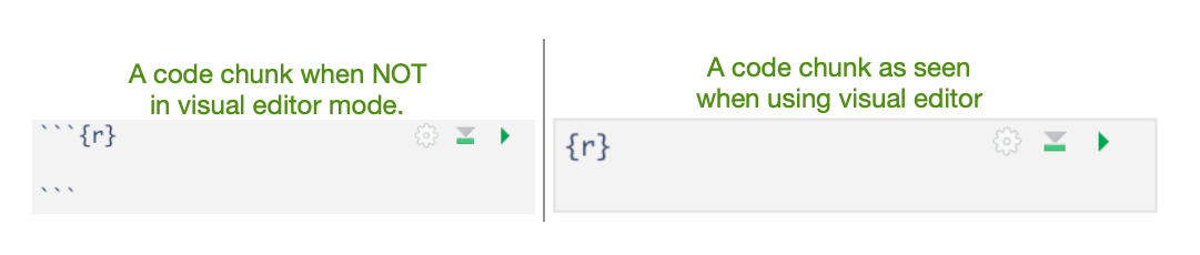
Other than our backticks ``` for code chunks that surround the code top and bottom, the only required piece is the specified language (r) placed between the curly brackets. This indicates that the language to read the code is R.
Fun fact: Other Programming Languages
Although we will (mostly) be using R in this workshop, it’s possible to use other programming or markup languages. For example, we have seen that we can use LaTeX code for equations. You can also use python and a handful of other languages, so if R is not your preferred programming, but you like working in the RStudio environment, don’t despair! Other options for languages include: sql, julia, bash, and c, etc. It should be noted however, that some languages (like python) will require installing and loading additional packages.
Add a Code Chunk
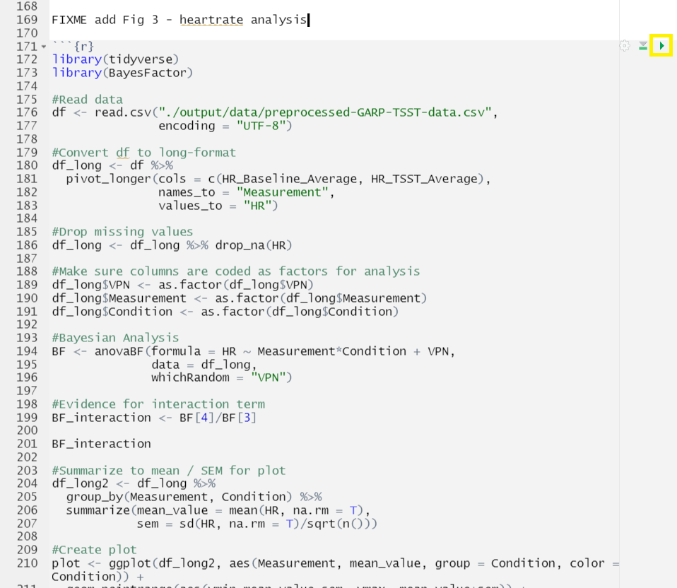
Ok, let’s add some code! There are already some plots included in our code but as static images. This time, we are going to opt to add these plots as code chunks - which are also more reproducible and easier to update. This is because, as with our inline code, this assures that if there are any changes to the data, the plots update automatically. This also makes our life easier because when there’s a change we don’t have to re-generate plots, save them as images and then add them back in to our paper. This will potentially help prevent version errors as well! So we’re actually going to go ahead and add a few plots with code chunks. We’ll start by typing our our starting backticks & r between curly brackets. (in your own workflow you may want to add the ending three backticks as well so you don’t forget after adding your code - it’s a common mistake):
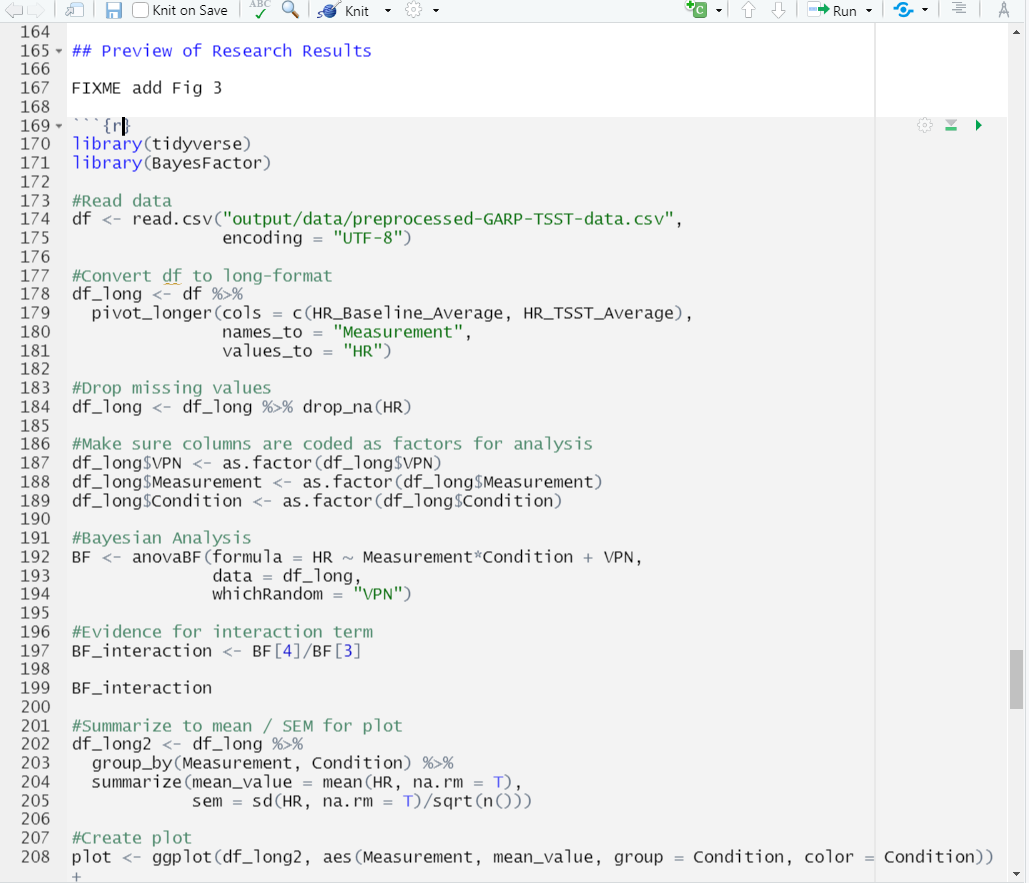
Now, let’s open our 03_HR_analysis.R script in our code folder. Copy the code and paste it in between the two lines with backticks and {r} in our DataPaper-ReproducibilityWorkshop.rmd file.
Tip:
There’s actually a button you can use in the RStudio menu to generate the code chunks automatically. Automatic code chunk generation is available for several other languages as well. Also, you can use the keyboard shortcut
ctrl+alt+Ifor Windows andcommand+option+Ifor Mac.
Now, to check to make sure our code renders, we could click the “knit” button as we have been doing. However, with the code chunks we have other opportunities for rendering.
1) Knit button - knitting will automatically run the code in all code chunks
2) Run from code chunk (green play button on the right top corner)
3) Run menu
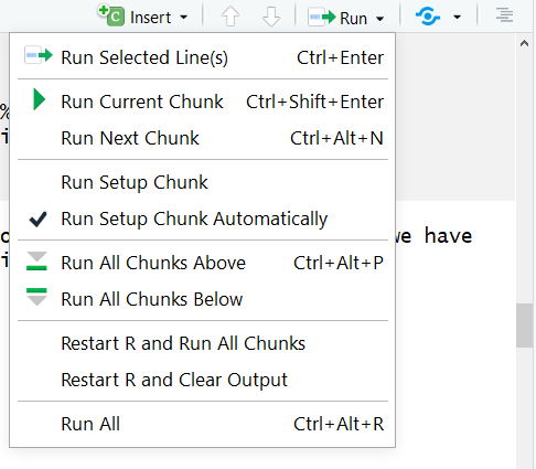
4) Keyboard shortcuts:
| Task | Windows & Linux | macOS |
|---|---|---|
| Create a code chunk | Ctrl + Alt + I | Cmd + Option + I |
| Run all chunks above | Ctrl+Alt+P | Command+Option+P |
| Run current chunk | Ctrl+Alt+C | Command+Option+C |
| Run current chunk | Ctrl+Shift+Enter | Command+Shift+Enter |
| Run next chunk | Ctrl+Alt+N | Command+Option+N |
| Run all chunks | Ctrl+Alt+R | Command+Option+R |
| Go to next chunk/title | Ctrl+PgDown | Command+PgDown |
| Go to previous chunk/title | Ctrl+PgUp | Command+PgUp |
Time to Knit!
Use one of the above options to run your code.
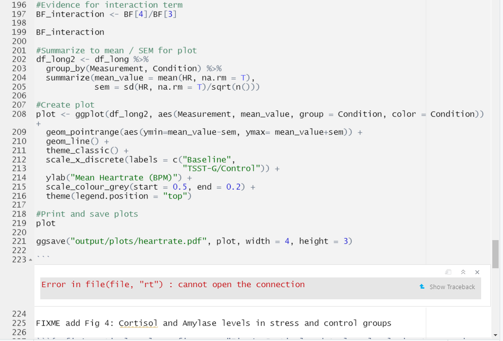
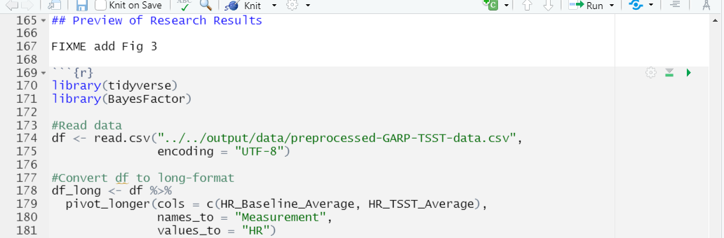
Hmmmm… we got an error while trying to run our code. That’s because our code contains a relative path to read in the data file, but now we’re running the code from the rmd document which is in a different directory so we will need to update the file path.
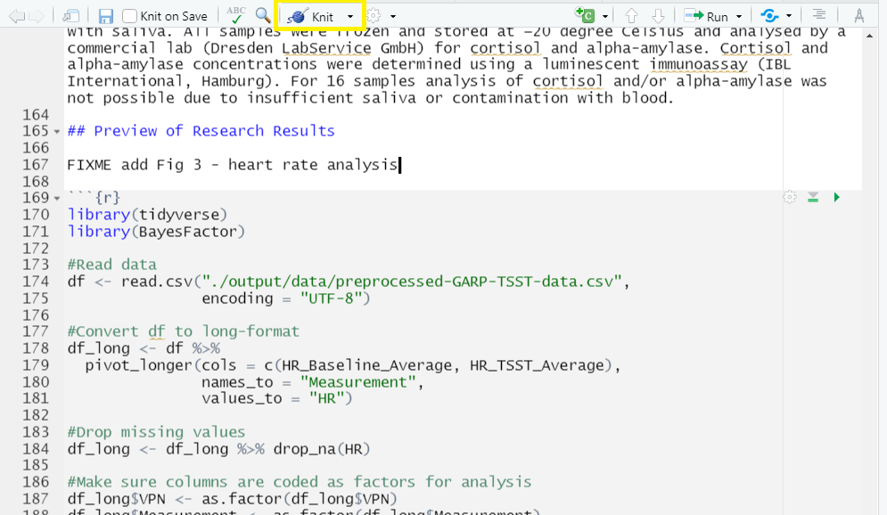
Update the file path from: "output/data/preprocessed-GARP-TSST-data.csv" to "../../output/data/preprocessed-GARP-TSST-data.csv"
Time to Knit!
Let’s try that again
Ooof! That output doesn’t look great.. we’ve got a bit more work to do.

let’s see about fixing that with code chunk rendering options.
Code Chunk Options, Names and Captions (oh my!)
Name Your Code Chunk
While not necessary for running your code, it is good practice is to give a name to each code chunk and allows for more advanced options (such as cross-referencing) to work with your rmd files later on:
{r chunk-name}
Some things to keep in mind
- The chunk name is the only value other than r in the code chunk options that doesn’t require a tag (i.e.
echo =) - The chunk label has to be unique (i.e.you can’t use the the same name for multiple chunks)
We’ll see in a bit where this code chunk label comes in handy. But, for now let’s go back and give our first code chunk a name:
{r fig3-heartrate}
Tip: Don’t use spaces, periods or underscores in code chunk labels
Try to avoid spaces, periods (.), and underscores (_) in chunk labels and paths. If you need separators, you are recommended to use hyphens (-) instead. For example, setup-options is a good label, whereas setup.options and chunk 1 are bad; fig.path = ‘figures/mcmc-‘ is a good path for figure output, and fig.path = ‘markov chain/monte carlo’ is bad. See more at: https://yihui.org/knitr/options/
Code Chunk Options
There are over 50 different code chunk options!!! Obviously we will not go over all of them, but they fall into several larger categories including: code evaluation, text output, code style, cache options, plot output and animation. We’ll talk about a few options for code evaluation, text output and plot output specifically.
Tip: Learn more about code chunk options
Find a complete list of code chunk options on Knitr developer, Yihui Xie’s, online guide to knitr. Or, you can find a brief list of all options on the R Markdown Reference guide on page 3 accesible through the RStudio Interface by navigating to the main menu bar
Help > Cheat Sheets > R Markdown Reference Guide.
The chunk name is the only value other than r in the code chunk options that doesn’t require a tag (i.e. the “= VALUE” part of option = VALUE). So these chunk options will always require a tag whose syntax looks like:
{r chunk-label, option = VALUE}
the option always follows the code chunk label (don’t forget to add a , after the label either).
Some common options:
results = (logical or character) text output of the code can be hidden (hide or FALSE), or delineated in a certain way (default ‘markup’).
eval = (logical or numeric) TRUE/FALSE to evaluate (or not) or a numeric value like c(1,3) (only evaluate expressions 1 and 3).
echo = (logical or numeric - following the same rules as above) whether to display source code or not.
warning = (logical) whether to display the warnings in the output (default TRUE). FALSE will output warnings to the console only.
include = (logical) whether to include the chunk output in the output document (default TRUE).
message = (logical) whether or not to display messages that appear when running the code (default TRUE).
CHALLENGE 9.1 - Rendering Codes
How will some hypothetical code render given the following options?
{r global-chunk-challenge, eval = TRUE, include = FALSE}SOLUTION
The expressions in the code chunk will be evaluated, but the outputed figures/plots will not be included in the knit document.
When might you want to use this?
If you need to calculate some value or do something on your dataset for a further calucation or plot, but the output is not important to be included in your paper narrative.
CHALLENGE 9.2 - add options to your code
Add the following options to your code:
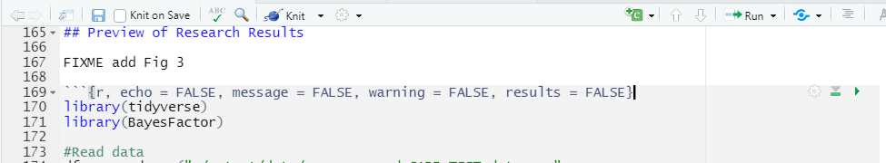
echo = FALSE, message = FALSE, warning = FALSE, results = FALSEWhat will this do?
SOLUTION
These options mean the source code will not be printed in the knit html document, messages from the code will not be printed in the knit html document, and warnings will not be printed in the knit html document (but will still output to the console). Plots, figures or whatever is printed by the code WILL show up in the final html document.
Caption your figure output from code chunks:
Again, this is an optional feature, but if you need (or want) to add captions to your publication, it is straightforward to do in code chunks.
The caption information also resides between your brackets at the beginning of the chunk: {r}
the tag is fig.cap followed by a = and the captions within quotes "caption for figure"
Challenge 9.3: Add a caption to Figure 3
Let’s add a caption to our heartrate figure. Add the caption:
“Fig 3: Mean heart rate of stress and control groups at baseline and during intervention.”
Solution
so, you should end up with the following in your code chunk:
{r fig3-heartrate, echo = FALSE, message = FALSE, warning = FALSE, results = FALSE, fig.cap = "Fig 3: Mean heart rate of stress and control groups at baseline and during intervention."}
Let’s knit one more time to see if our figure outputs how we’d like and has a caption.
Time to Knit!
Let’s try that again
Now that we’ve named and adjusted the rendering for our first figure, let’s add another, but instead of copy/pasting an r script into our rmd document we will use a more elegant solution.
Key Points
Knitr will render your code and R markdown-formatted text and output your document format of choice
Code chunks are runable piece of R code. Each time you knit the document, calculations and plots will be run and displayed
Options for code chunks can be set at the individual level or at the global level
Global Code Chunk Settings & Inline Code
Overview
Time: 50 minObjectives
Learn how to source external scripts to run within an rmd document.
Learn about using global knitr options and global chunk options
Learn the syntax for inline code
Run Code from an external script in a code chunk
Let’s add another figure generated from code. This time around let’s see how to run code in a code chunk from an external R script instead of unelegantly copying and pasting the code from a R script to a code chunk in our .rmd.
There are at least a few benefits to running code in this modular fashion instead of copy/pasting:
- Automatic updates: if the code gets updated in the R script, it automatically be updated in the rmd document as well.
- Readability: calling code externally only takes several lines of code - versus copy/pasting 50+ lines of code from our scripts.
- Less fussing with relative paths* - we had to change the code slightly in the first example to update the file path to the data set, with this method we won’t have to modify the source code.
*unfortunately you will never be free of relative paths, but you can make it a bit easier on yourself.
First, find the FIXME in the rmd document for Fig 4 (ctrl-f “Fig 4”). We need to add the code for the hormone analysis.
Add your code chunk:
Now, within the chunk add the code:
# run the code from 02_hormone_analysis.R in the code directory
source("../../code/02_hormone_analysis.R", local = knitr::knit_global())
# display the plot created by code in 02_hormone_analysis.R
plot
Time to Knit!
Let’s see if our code worked from an external script
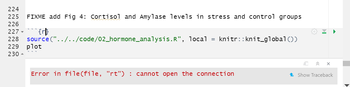
Shoot, we got an error and it looks familiar… another file path error. That’s because the code we are calling from within the rmd document contains file paths to read and save the data that are relative to the code directory where the 02_hormone_analysis.R resides so the paths aren’t correct when run from the .rmd file. Yesh! All sorts of relative path chaos.
What do we do now? We could go into the 02_hormone_analysis.R file and change the relative paths to work with the .rmd file, but then they won’t run correctly on their own. Also, this wouldn’t accomplish our goal of streamlining our plot generation by running an external script. Ugh, what can we do???
Well, there is a solution to this as well! (As with most every obstacle you run into with R). That solution is to change the working directory of our rmd document - to do that we will first introduce Global knitr options.
Tip: Many ways to run external code
There are at least 3-4 methods one can use to run external code, the best choice may just depend on the context or on your personal preference. All are a bit awkward because of relative paths, but better than copy/pasting code from elsewhere in your project (in our humble opinion):
- source() – see more at bookdown.org
- sys.source() – see more at bookdown.org
- knitr::read_chunk() – see more at stackoverflow
- code() *in
{r}header see more at stackoverflow
- another helpful page: http://zevross.com/blog/2014/07/09/making-use-of-external-r-code-in-knitr-and-r-markdown/
Global Knitr options
Benefits of global knitr options:
- Set working directory so file paths (for code chunks) can be relative to the root instead of our .Rmd file
- Code chunk options that can be applied consistently for the whole document
- Load libraries and data once at the beginning of the doucment instead of in each code chunk (more concise and less rendering time)
Set working directory to project directory:
Ok, so let’s fix these path issues we get when we try to run externally sourced code. The definition of relative paths is that they are relative to your current document or working directory. So we are having issues with connections trying to read our data files because the R scripts in our code directory (../ to get to the ‘root’ or .Rproj directory) are in a different location relative to our rmd document (../..). What we want to do is direct RStudio to change the default working directory for the rmd document from the directory where the document is located to the project directory (which is the root directory of our project where the .Rproj file is located). We actually have several methods to do it.
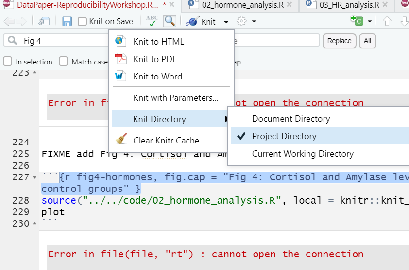
The first option is easy - we click the menu next to the knit button and change Knit Directory to Project Directory. *NOTE this is a bit awkward because it ONLY changes the root directory for the code chunks NOT our narrative portions (think image links and inline code).
The second option requires a bit of code, but will overall be more reproducible (because it’s not dependent on your personal RStudio IDE settings) This is a setting option in our global knitr settings:
We will now navigate back up to the top of our .rmd document, right after the yaml. Here, we will add a new code chunk with the label setup and the options echo = FALSE (we don’t need this code printed out in our final document!). Then, we’ll add the following line of code:
knitr::opts_knit$set(root.dir = rprojroot::find_rstudio_root_file())
*notice this code uses one of our pre-installed packages rprojroot
Finally, let’s adjust the path in the source() function after our working directory change.
source("../../code/02_hormone_analysis.R) to source("code/02_hormone_analysis.R")
Looks neater already!
Ok, now that we’ve done that we’ll have to go back and fix the Figure 3 code and the inline code we added earlier so it runs properly since the working directory has changed.
Challenge 9.4
Fix the relative path in the Figure 3 code so that the chunk will run properly. Hint: We changed the working directory from the directory where the
rmddocument livesreport/sourceto the project directory, aka the ‘root directory’Solution
There are two options:
- change the relative path on the line read.csv() from
../../output/tooutput/- delete the code from the code chunk and run the code from the external R script as with Figure 4.
Challenge 9.5
Fix the relative path in the inline code so that the chunk will run properly. Hint: We changed the working directory from the directory where the
rmddocument livesreport/sourceto the project directory, aka the ‘root directory’.Solution
Change the relative path for the inline code in the section of the paper that describes the bronars simulation data from
r bronars_data <- read.csv("../../data/bronars_simulation_data.csv")tor bronars_data <- read.csv("data/bronars_simulation_data.csv")
Note: setting the knit directory globally with opts_knit$set
Setting the knit directory to the project directory with the setup code chunk as we just did adjusts the working directory for all code in the R Markdown document (code chunks and inline code), but NOT for any markdown text elements (images and hyperlinks).
Time to Knit!
Let’s make sure all our file paths are correct and our code runs without errors.
Now, we can have some more fun with global options:
Global Code Chunk Options:
With our plots we set the options for each chunk individually. However, we may end up with quite a few code chunks in our paper and it might be a lot of work to keep track of what options we’re using throughout the paper. We can automate setting options by adding a special code chunk at the beginning of the document. Then, each code chunk we add will refer to those “global” options when it runs.
To set global options that apply to every chunk in your file, we will call knitr::opts_chunk$set() in a new code chunk right after our yaml header (name the new code chunk setup.
Knitr will treat each option that we add to this call as default settings for all code chunks. However, we will need to set the options for this code chunk in the first place! so we’ll use the options from our first code chunk. In the () after the knitr::opts_chunk$set() add the options:
knitr::opts_chunk$set(echo = FALSE, message = FALSE, warning = FALSE, results = FALSE)
Alright! That takes care of Fig 4 as well as Fig 3. Now we could go back and remove the options we set in the individual code chunks since we’ve set the global options in the document instead (however, if we left them it would render just the same.)
Time to Knit!
Again, let’s make sure our global options look right by knitting.
Tip: Overiding global options
What if you want most of your code chunks to render with the same options (i.e. echo = FALSE), but you just have one or two chunks that you want to tweak the options on (i.e. display code with echo = TRUE)? Good news! The global options can be overwritten on a case by case basis in each individual code chunk.
CHALLENGE 9.5 (optional) global & individual code chunk options
How would appear in our html document if we knit a code chunk with the following options?
{r challenge-5, warning = TRUE, echo = TRUE}…considering the global chunk settings were as listed:
knitr::opts_chunk$set(echo = FALSE, include = FALSE)SOLUTION
In this case, the global settings are set so neither the code nor the output will display. However, the individual chunk reverses the echo setting so the code will display, and it also indicates that any warnings the code renders should output too. The outputs of the code would still not be displayed (include = FALSE) The hypothetical situation for this configuration may be for debugging while writing the rmd document.
Before we lose track of where we were with editing up our second code chunk, let’s finish it up by going back and adding a caption and name:
Challenge 9.6: Add chunk name and caption to Figure 4
Add the caption:
Fig 4: Cortisol and Amylase levels in stress and control groupsAdd the name:fig4-hormonesSolution
{r fig4-hormones, fig.cap = "Fig 4: Cortisol and Amylase levels in stress and control groups" }
Globally load data and packages
We can actually make our lives easier in one other way too. So far we’ve loaded the library tidyverse and data frame data1 we need in the first code chunk. Now if we want to replace, say Figure 3 (which we will do next), we would load tidyverse and the data for Figure 3, meaning we would be loading tidyverse for a second time unnecessarily. This is because once libraries and data are loaded they are available for the rest of the rmd document.
Instead, we can load libraries and data at the beginning of our document which makes it available for all other figures or calculations and lets us avoid repetition. This also makes it easier for us to keep track of all the libraries and data we need to use in any given document. If anything needs to be tweaked, we don’t need to search through every code chunk in our rmd document to make a change.
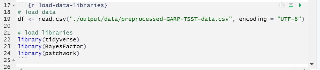
# load data
df <- read.csv("./output/data/preprocessed-GARP-TSST-data.csv", encoding = "UTF-8")

# load libraries
library(tidyverse)
library(BayesFactor)
library(patchwork)
It’ll look like the following:
At this point we could go back through our R scripts and comment out (or delete) the beginning sections where we load the data and libraries. That will save some time for the rmd document to render, because the data and libraries will only load once instead of twice. You can imagine that the more code chunks you have the more time taking this step would save. Bonus that this also works to load the data before it is called in inline code as well!
Inline Code
What if you only need to make a quick calculation and adding a code chunk seems a little overkill?
You can also include r code directly in your the text portion of your document. Say you are discussing some of the summary statistics in your manuscript, R Markdown makes this possible through HTML/LaTeX inline code which allows you to calculate simple expressions integrated to your narrative. Inline code enables you to insert r code into your document to dynamically updated portions of your text. In other words, if your data set changes for any reason the code will automatically update the calculation specified.
This can be helpful when referring to specific variables on your data. For example, you should include numbers that are derived from the data as code not as numbers. Thus, rather than writing “The CSV file contains choice consistency data for 10.000 simulated participants” (FIXME8), replace the static number with a bit of code that, when evaluated, gives you a dynamic number if anything changes on your dataset. Please note that this insertion is not included in the visual editor, so we need to do write an expression, for example:
The CSV file contains choice consistency data for r nrow(bronars_simulation_data.csv) simulated participants.
When you knit you might get an error. Any idea why? That is because we need to make sure to import the dataset we are referring to and call it in R Markdown before the inline code can work. Let’s follow this process by including:
r bronars_simulation_data <- read.csv("../../data/bronars_simulation_data.csv")
Time to Knit! If you update your dataset this value will match the number of rows.
CHALLENGE 6.1 - Adding inline code
Suppose we would like to add some information to the sentence we have just adjusted in our manuscript. We would like to include the average for the variable violation_count present in the same dataset. Which inline code we would have to add to following sentence?
The CSV file contains choice consistency data for `
r nrow(bronars_simulation_data.csv)` simulated participants, that have been used to determine the power of our food-choice task design to detect choice consistency violations, which averaged `enter inline code here`. What inline code would you enter? What number would replace the inline code?Tip: we will need to use a
dataset$variablesyntax!Solution:
`
r mean(bronars_simulation_data$violation_count)` 5.3924
Important Note:
Make sure the file you are calling is in the right subdirectory and your working directory is set appropriately.
More on inline codes:
R Markdown will always display the results of inline code, but not the code. Inline expressions do not take knitr options.
Tip: Yaml chunk options
We can also tweak some settings in our yaml which changes how code chunks are displayed. We’re not going to get into this in the workshop, but many of the same options you set in your global code chunk settings are also configurable in the yaml.
Adjust rendered html output directory
Ok, we’ll adjust one thing in the yaml. You know how we said it’s good practice to have code and output from the code in separate directories? Well, the html file that renders from our .rmd file outputs to the same report/source directory. So that violates our standards. It might not be the end of the world, but let’s see how to change the directory that R Markdown documents output to after knitting.
This is unfortunately more difficult that one would like, but we can use the following code in the yaml to create a custom function that changes the output directory for the .rmd file.
The code for our documet is as follows:
knit: (function(rmdFile, encoding) {
      out_dir <- '../output';
      rmarkdown::render(rmdFile,
                        encoding=encoding,
                        output_file=file.path(dirname(rmdFile),
                        out_dir,
                        'DataPaper-ReproducibilityWorkshop.html'))})
Simply copy and paste it in to the yaml.
Key Points
Options for code chunks can be set at the individual level or at the global level
Use a setup chunk at the beginning of your document to declare global options
Use a chunk at the beginning of your document to load libraries and data globally to make your document more effiecient.
Bibliography & Citations
Overview
Time: 25 minObjectives
Inserting citations and listing bibliography in an R Markdown file.
Changing citation styles.
Customizing how citations and bibliography are displayed.
Why citing?
Correctly citing and attributing publications is key to academic writing. Older versions of RStudio require Pandoc’s citation syntax to render bibliographies correctly. We won’t be covering this approach extensively in this workshop, since the new visual editor has made this process much more simple. You can refer to our previous workshop on R Markdown pre-visual editor for more information.
The new visual editor in RStudio 1.4 has made citations and cross-referencing much easier, by offering different options for referencing various types of sources. Before getting into these different features, let’s first learn how you can call the citation window dialog on Rstudio and how to navigate these different options.
Calling Citation Options on Rstudio
After placing your cursor where you want to insert the citation you can either click the @ icon in the toolbar, or select Insert, and from the drop down menu choose Citation. Alternatively you can use the keyboard shortcut ⇧⌘ F8 on Mac, or Ctrl+Shift+F8 for Windows.
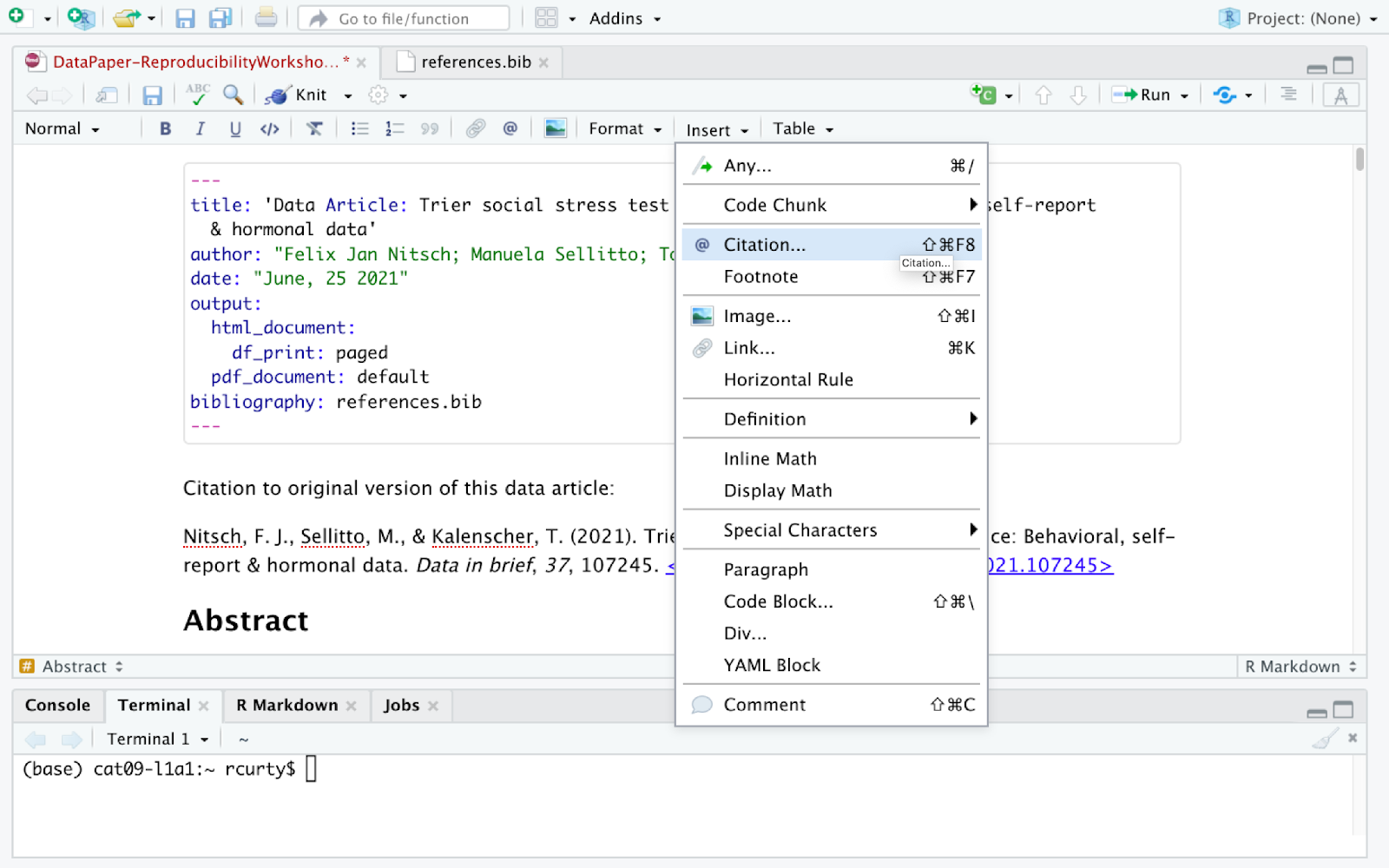
The citation window will display different options for inserting citations, You can either find items listed in your own sources through your Bibliography folder (you should have one already in your project folder provided by us), your Zotero Library(ies) if you have the reference manager installed in your computer, or even use the lookup feature to search for publications by DOI (Digital Object Identifier), Crossref, DataCite, or PubMed ID.
Understanding How Rstudio Stores and Organizes Citations
Have you noticed that the YAML header contains “bibliography: references.bib”. Any idea why? Well, that’s because on our paper template we have some existing citations, and a references.bib file in our project folder. Rstudio adds that automatically to the YAML once you cite the first item to your manuscript. But let’s first open the references.bib file and understand how citations are presented there:
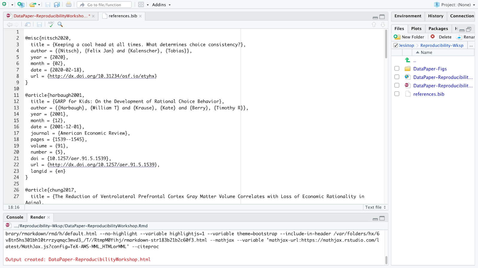
A file with the BIB file extension is a BibTeX Bibliographical Database file. It’s a specially formatted text file that lists references pertaining to a particular source of information. They’re normally seen only with the .BIB file extension but might instead use .BIBTEX. BibTeX files might hold references for things like research papers, articles, books, etc. Included within the file is often an author name, year, title, page number, and other related content. Each item can be edited, in case there is any metadata incorrect or missing.
Most citation and reference management tools such as Refworks, Endnote, Mendeley and Zotero, as well as some search engines (e.g. Google Scholar), most scientific databases, and our UCSB library catalog allow us to export citations as .bib BibteX files. These files are used to describe and process lists of references, mostly in conjunction with LaTeX documents. Each .bib file has a citation key or ID preceded by an @, which uniquely identifies each item. Citation keys can be customized as we will learn in a bit, but be advised that your manuscript will render citations correctly only if you have the cited item corresponding to its exact key.
Inserting Citations
Note that we have different blocks in this file starting with a @ and ending with a curly bracket {, each one representing a unique citable source. We will be adding now a new item using the DOI lookup function so that you can see how the magic works!
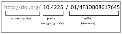
Let’s assume you want to include a citation in the first line of the Value of the Data section, because you would like to provide some reference of how the salivary cortisol technique has been used in research. So let’s click where we want to insert the citation, call the citation function and lookup for the following DOI: https://doi.org/10.1016/B978-012373947-6.00334-2
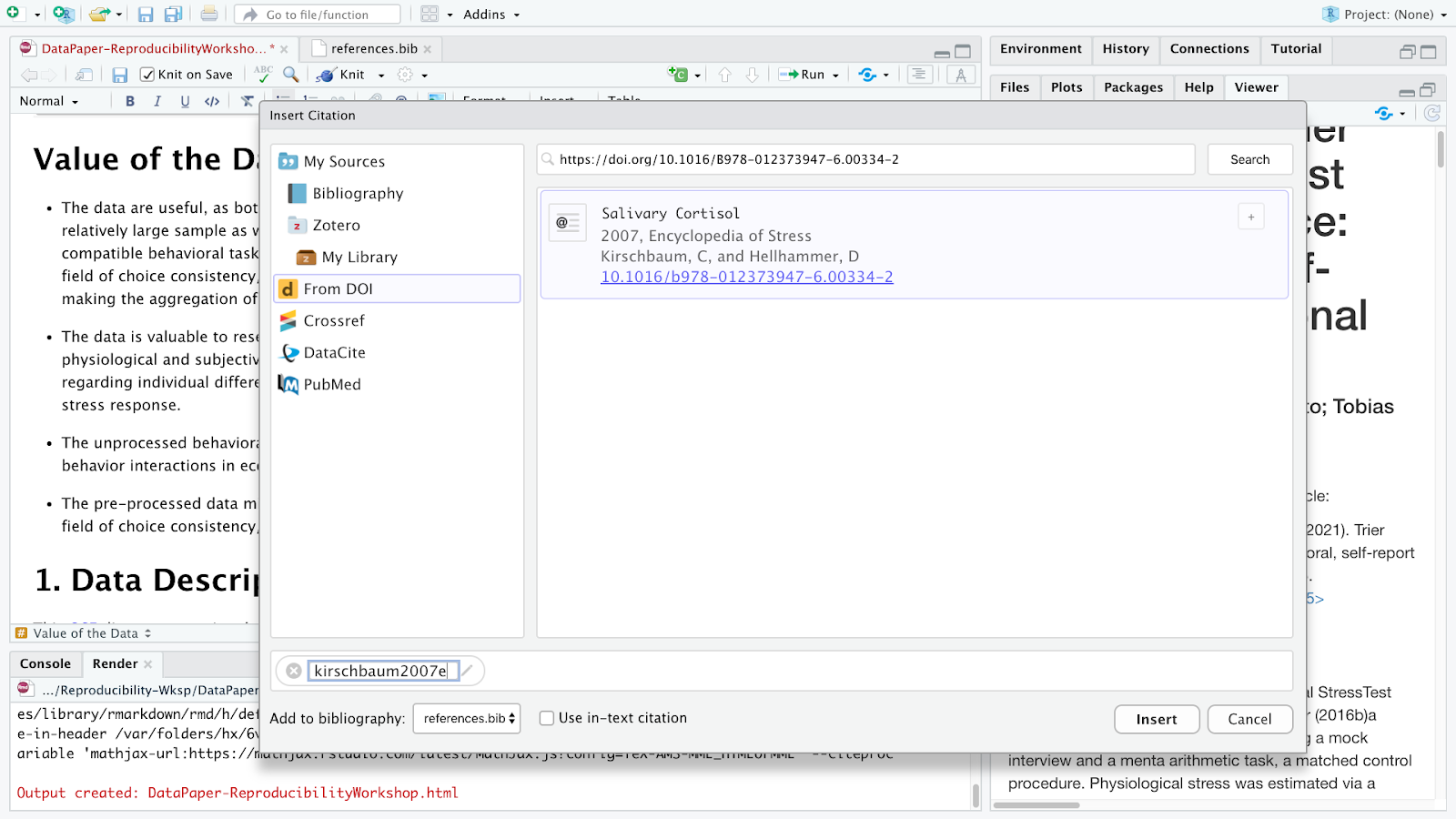
The DOI lookup uses the persistent identifier which connects to the DOI resolver service and retrieves the .bibtex file with resource metadata1. You should insert the whole DOI address, including the resolver service, the prefix and the suffix which is specific to the resource as illustrated below:
Rstudio will search the DOI API and list the only matching result and you can insert it. After confirming this is the citation you would like to include, you can modify the key, if you would like to simplify it, and also choose if you would like to insert it as a in-text citation, meaning you would like to have the last name of the author(s) followed by a page number enclosed in parentheses. i.e., Kirschbaum and Hellhammer (2007), but in this case, we will uncheck that option since we won’t include authors as part of the narrative. Instead we would like to insert a parenthetical citation, where authors and year will be displayed inside the parentheses such as (Kirschbaum and Hellhammer 2007). You may insert more than one citation by selecting multiple items.
This item will be automatically listed in your Bibliography folder, and if you want to cite this same item again you can type @ and the first letters of the item name which will be auto-completed by Rstudio. For parenthetical citations you will have to type the key between brackets and for in-text narrative citations, you only need to type in the key.
Note that when you hover over the citation, you will preview the full reference for the cited item that will be listed at the bottom of the manuscript. This feature helps you to identify if you have to edit anything in the .bib file your citation is calling. Also, note that all citations will be included at the end of your document under a reference list.
Challenge 8.1 - Insert a Citation Using the DOI Lookup Function
Following the same process described, insert a parenthetical citation to the publication “Welcome to the tidyverse” (https://doi.org/10.21105/joss.01686) where there is a mention to this package in the data paper. Look for:
insert citation hereSolution
[@wickham2019]
(Wickham et al., 2019)
Inserting citations using Crossref, DataCite or PubMed follows a very similar process to the DOI process, however; to search on their APIs you will need to input information accordingly. For Crossref, you may use keywords and author information to identify an item (e.g., Cortisol Stress Oken) and Rstudio will connect to Crossref search and provide related results, often not as specific as the DOI search, for cases you know exactly what you are looking for. DataCite allows searches by persistent identifiers or keywords, while PubMed searches exclusively in biomedical literature indexed in the database. If you have the PMID (PubMed reference number), which is uniquely assigned by the NIH National Library of Medicine to papers indexed in PubMed, similarly to the DOI search, it will save you time.
Editing Metadata & Citation Key
Not all citations are perfect shape when in import them. Sometimes we will need to perform some adjustments (e.g., include missing metadata, move content to another metadata field). If needed, we can do so by modifying the .bib file. As briefly mentioned, you can also edit citation keys. By default, most citation keys will have the first author last name or the first word of the title (if no authors), followed by the year of publication. You may consider editing the citation key in case you want to simplify the entry and speed up the autocomplete option. If you choose to do so, you can simply click on the key in the .bib file and edit it. Please be advised to use this option with caution, and to update citations to match the .bib file.
Changing Citation Styles
You might have noticed that all citations are inserted in a specific style. Can you guess which one? If you answered Chicago that is correct! By default, Rstudio via Pandoc will use a Chicago author-date format for citations and references. To use another style, you will need to specify a CSL (Citation Style Language) file in the csl metadata field in the YAML.
But how can you identify which CSL you should use? You can find required formats on the Zotero Style Repository, which makes it easy to search for and download your desired style.
Download the format you wish to use and call it out in the YAML. Let’s try it together! Go to the Zotero Style repo and select American Psychological Association 7th edition. You will notice that it will automatically download a apa.csl file. Make sure to save it to your project folder in report/source folder. In the YAML we have to call the exact name of the file preceded by “csl:”
csl: apa.csl
Save and knit the document to see how citations and references have changed. This same process could be followed for any citation style required by the university, the journal or conference you are planning to submit your manuscript to.
Challenge 8.2 - Changing the Citation Style
How can you go back to using Chicago Style?
Solution
You can either delete the csl information as it is set as the default, or call it in the YAML:
csl: chicago.csl
Adding Items to the References without Citing them
All cited items will be listed under the section References which you created before while practicing headings and subheadings. Items will be placed automatically in alphabetical order for most citation styles. However, there might be cases that you will be referencing supporting literature which you have not necessarily cited in the document.
By default, the bibliography will only display items that are directly referenced in the document. If you want to include items in the bibliography without actually citing them in the body text, you can define a dummy nocite metadata field in the YAML and put the citations there.
nocite: |
  @item1, @item2
To demonstrate that I will add a new bibtex from my Google Scholar Library and specify the @key in the YAML. Note that this will force all items added in the YAML to be displayed in the bibliography.
Let’s try!
Challenge 8.3 - Adding references you have not cited
Find and remove the existing in-text citation to
@peirce2007, but list it out in the reference section.Solution
You can either delete the csl information as it is set as the default, or call it in the YAML:
nocite: |
 @peirce2007
Important Info:
Does the indentation matter? Yes, you have to indent at least one space and the citation key should turn green to work.
In case you are including a citation tonocitethat you have not cited in the document, you have to make sure first that the bib file is in your Bibliography folder.
Time to Commit!
Make sure to commit your changes to GitHub. Add your changed files and commit with the following message: “Added Bibliography”
Key Points
Rstudio supports different lookups strategies to easy the citation process.
Rstudio supports different citation styles.
The YAML can be ajusted to display uncited items in the reference list.